Anomaly Detection (Snowflake ML Functions)
Overview
Anomaly detection is the process of identifying outliers in data. The anomaly detection function lets you train a model to detect outliers in your time-series data. Outliers, which are data points that deviate from the expected range, can have an outsized impact on statistics and models derived from your data. Spotting and removing outliers can therefore help improve the quality of your results.
Note
Anomaly Detection is part of Snowflake’s suite of business analysis tools powered by machine learning.
Detecting outliers can also be useful in pinpointing the origin of problems or deviations in processes when there is no obvious cause. For example:
- Determining when a problem started to occur with your logging pipeline.
- Identifying the days when your Snowflake compute costs are higher than expected.
Anomaly detection works with either single-series or multi-series data. Multi-series data represents multiple independent threads of events. For example, if you have sales data for multiple stores, each store’s sales can be checked separately by a single model based on the store identifier.
The data must include:
- A timestamp column.
- A target column representing some quantity of interest at each timestamp.
Note
Ideally, the training data for an Anomaly Detection model has time steps at equally spaced intervals (for example, daily). However, model training can handle real-world data that has missing, duplicate, or misaligned time steps. For more information, see Dealing with real-world data in Time-Series Forecasting.
To detect outliers in time-series data, use the Snowflake built-in class ANOMALY_DETECTION (SNOWFLAKE.ML), and follow these steps:
-
Create an anomaly detection object, passing in a reference to the training data.
This object fits a model to the training data that you provide. The model is a schema-level object.
-
Using this anomaly detection model object, call the <model_name>!DETECT_ANOMALIES method to detect anomalies, passing in a reference to the data to analyze.
The method uses the model to identify outliers in the data.
Anomaly detection is closely related to Forecasting. An anomaly detection model produces a forecast for the same time period as the data you’re checking for anomalies, then compares the actual data to the forecast to identify outliers.
About the Algorithm for Anomaly Detection
The anomaly detection algorithm is powered by a gradient boosting machine (GBM). Like an ARIMA model, it uses a differencing transformation to model data with a non-stationary trend and uses auto-regressive lags of the historical target data as model variables.
Additionally, the algorithm uses rolling averages of historical target data to help predict trends, and automatically produces cyclic calendar variables (such as day of week and week of year) from timestamp data.
You can fit models with only historical target and timestamp data, or you may include exogenous data (variables) that might have influenced the target value. Exogenous variables can be numerical or categorical and may be NULL (rows containing NULLs for exogenous variables are not dropped).
The algorithm does not rely on one-hot encoding when training on categorical variables, so you can use categorical data with many dimensions (high cardinality).
If your model incorporates exogenous variables, you must provide values for those variables at timestamps in the future when detecting anomalies. Appropriate exogenous variables could include weather data (temperature, rainfall), company-specific information (historic and planned company holidays, advertisement campaigns, event schedules), or any other external factors you believe may help predict your target variable.
Optionally, individual historical rows can be labeled as anomalous or non-anomalous by using a separate Boolean column.
A prediction interval is an estimated range of values within an upper bound and a lower bound in which a certain percentage of data is likely to fall. For example, a 0.99 value means that 99% of the data likely appears within the interval. The anomaly detection model identifies any data that falls outside of the prediction interval as an anomaly. You can specify a prediction interval or use the default, which is 0.99. You may want to set this value to be very close to 1.0; 0.9999 or even closer.
Important
From time to time, Snowflake may refine the anomaly detection algorithm. Such improvements roll out through the regular Snowflake release process. You cannot revert to a previous version of the feature, but models you created with a previous version continue to use that version for anomaly detection.
Limitations
- You cannot choose or adjust the anomaly detection algorithm. In particular, the algorithm does not provide parameters to override trend, seasonality, or seasonal amplitudes; these are inferred from the data.
- The minimum number of rows for the main anomaly detection algorithm is 12 per time series. For time series with between 2 and 11 observations, anomaly detection produces a “naive” result in which all predicted values are equal to the last observed target value. For the labeled anomaly detection case, the number of observations used is the number of rows where the label column is false.
- The minimum acceptable granularity of data is one second. (Timestamps must not be less than one second apart.)
- The minimum granularity of seasonal components is one minute. (The function cannot detect cyclic patterns at smaller time deltas.)
- The “season length” of autoregressive features is tied to the input frequency (24 for hourly data, 7 for daily data, and so on).
- Anomaly detection models, once trained, are immutable. You cannot update existing models with new data; you must train an entirely new model. Models do not support versioning. Generally, you should retrain models on a regular cadence, such as once a day, once a week, or once a month, depending on how frequently you receive new data, to help the model keep up with changing trends.
- This feature only detects anomalies in the test data; it cannot detect anomalies in the training data. Furthermore, timestamps in the test data must all be greater than timestamps in the training data. Ensure that the training data covers a typical period free of actual outliers, or label known outliers in a Boolean column.
- You cannot clone models or share models across roles or accounts. When cloning a schema or database, model objects are skipped.
- You cannot replicate an instance of the ANOMALY_DETECTION class.
Preparing for Anomaly Detection
Before you can use anomaly detection, you must:
- Select a virtual warehouse in which to train and run your models.
- Grant the privileges to create anomaly detection objects.
You might also want to modify your search path to include SNOWFLAKE.ML.
Selecting a Virtual Warehouse
A Snowflake virtual warehouse provides the compute resources for training and using your machine learning models for this feature. This section provides general guidance on selecting the best size and type of warehouse for this purpose, focusing on the training step (the most time-consuming and memory-intensive part of the process).
Training on Single-Series Data
For models trained on single-series data, you should choose the warehouse type based on the size of your training data. Standard warehouses are subject to a lower Snowpark memory limit, and are more appropriate for training jobs with fewer rows or exogenous features. If your training data does not contain any exogenous features, you can train on a standard warehouse if the dataset has 5 million rows or less. If your training data uses 5 or more exogenous features, then the maximum row count is lower. Otherwise, Snowflake suggests using a Snowpark-optimized warehouse for larger training jobs.
In general, for single-series data, a larger warehouse size does not result in a faster training time or higher memory limits.
As a rough rule of thumb, training time is proportional to the number of rows in your time series. For example, on a XS
standard warehouse, with evaluation turned off (CONFIG_OBJECT => {'evaluate': False}), training on a
100,000-row dataset takes about 60 seconds, while training on a 1,000,000-row dataset takes about 125 seconds. With
evaluation turned on, training time increases roughly linearly by the number of splits used.
For best performance, Snowflake recommends using a dedicated warehouse without other concurrent workloads to train your model.
Training on Multi-Series Data
As with single-series data, choose the warehouse type based on the number of rows in your largest time series. If your largest time series contains more than 5 million rows, the training job is likely to exceed memory limits on a standard warehouse.
Unlike single-series data, multi-series data trains considerably faster on larger warehouse sizes. The following data points can guide you in your selection. Once again, all these times are done with evaluation turned off.
| Warehouse type and size | Number of time series | Number of rows per time series | Training time (seconds) |
|---|---|---|---|
| Standard XS | 1 | 100,000 | 60 seconds |
| Standard XS | 10 | 100,000 | 204 seconds |
| Standard XS | 100 | 100,000 | 720 seconds |
| Standard XL | 10 | 100,000 | 104 seconds |
| Standard XL | 100 | 100,000 | 211 seconds |
| Standard XL | 1000 | 100,000 | 840 seconds |
| Snowpark-optimized XL | 10 | 100,000 | 65 seconds |
| Snowpark-optimized XL | 100 | 100,000 | 293 seconds |
| Snowpark-optimized XL | 1000 | 100,000 | 831 seconds |
Detecting Anomalies
The inference step takes approximately 1 second to process 100 rows in the input dataset, regardless of warehouse size.
Granting Privileges to Create Anomaly Detection Objects
Training an anomaly detection model results in a schema-level object. Therefore, the role you use to create models must have the CREATE SNOWFLAKE.ML.ANOMALY_DETECTION privilege on the schema where the model is created, which allows the model to be stored there. This privilege is similar to other schema privileges like CREATE TABLE or CREATE VIEW.
Snowflake recommends that you create a role named analyst to be used by people who need to detect anomalies.
In the following example, the admin role is the owner of the schema admin_db.admin_schema. The
analyst role needs to create models in this schema.
To use this schema, a user assumes the role analyst:
If the analyst role has CREATE SCHEMA privileges in database analyst_db, the role can create a new schema
analyst_db.analyst_schema and create anomaly detection models in that schema:
To revoke a role’s model creation privilege on the schema, use REVOKE <privileges> … FROM ROLE:
Setting Up the Data for the Examples
The examples in the following sections use a sample dataset that contains daily sales for items in different stores along with daily weather data (humidity and temperature). The dataset also contains a column that indicates whether the day is a holiday.
- Execute the following statements to create a table named
historical_sales_datathat contains the training data for the model:
- Execute the following statements to create a table named
new_sales_datathat contains the data to analyze:
Training, Using, Viewing, Deleting, and Updating Models
Use CREATE SNOWFLAKE.ML.ANOMALY_DETECTION to create and train a model. The model is trained on the dataset you provide.
See ANOMALY_DETECTION (SNOWFLAKE.ML) for complete details about the SNOWFLAKE.ML.ANOMALY_DETECTION constructor. For examples of creating a model, see Detecting Anomalies.
Note
SNOWFLAKE.ML.ANOMALY_DETECTION runs using limited privileges, so by default it does not have access to your data. You must therefore pass tables and views as references, which pass along the caller’s privileges. You can also provide a query reference instead of a reference to a table or a view.
To create this reference, you can use the TABLE keyword with the table name, view name, or query, or you can call the SYSTEM$REFERENCE or SYSTEM$QUERY_REFERENCE function.
To detect anomalies, call the model’s <model_name>!DETECT_ANOMALIES method:
To select columns from the tabular output of the method, you can call the method in the FROM clause:
To view a list of your models, use the SHOW SNOWFLAKE.ML.ANOMALY_DETECTION command:
To remove a model, use the DROP SNOWFLAKE.ML.ANOMALY_DETECTION command:
To update a model, delete it and train a new one. Models are immutable and cannot be updated in place.
Detecting Anomalies
The following sections demonstrate how to use anomaly detection to detect outliers. These sections provide examples of detecting anomalies for a single time series, for multiple time series, with and without exogenous variables, with a user-defined prediction interval, and with a supervised (labeled) approach.
- Detecting Anomalies for a Single Time Series (Unsupervised)
- Training an Anomaly Detection Model with Labeled Data
- Specifying the Prediction Interval For Anomaly Detection
- Including Additional Columns for Analysis
- Detecting Anomalies in Multiple Series
Detecting Anomalies for a Single Time Series (Unsupervised)
To detect anomalies in your data:
- Train an anomaly detection model using historical data.
- Use the trained anomaly detection model to detect anomalies in historical or projected data. The timestamps in the test data must chronologically follow the timestamps in the training data. You need at least 2 data points to train a model, at least 12 for non-naive results, and at least 60 for non-linear results.
See ANOMALY_DETECTION (SNOWFLAKE.ML) for information on the parameters used in creating and using a model.
Training an Anomaly Detection Model
To create an anomaly detection model object, execute the CREATE SNOWFLAKE.ML.ANOMALY_DETECTION command.
For example, suppose that you want to analyze the sales for jackets in the store with the store_id of 1:
-
Create a view or design a query that returns the data for training the model for anomaly detection.
For this example, execute the CREATE VIEW command to create a view named
view_with_training_datathat contains the date and sales information: -
Create an anomaly detection object, and train its model on the data in that view.
For this example, execute the CREATE SNOWFLAKE.ML.ANOMALY_DETECTION command to create an anomaly detection object named
basic_model. Pass in the following arguments:This example passes in a reference to a view as the INPUT_DATA argument. The example uses the TABLE keyword to create the reference. As an alternative, you can call SYSTEM$REFERENCE to create the reference.
The purpose of the label column is to tell the model which rows are known anomalies. Because this example uses unsupervised training, you do not need to use the label column. Pass an empty string as the name of the label column.
Tip
If you don’t want to create a view for the INPUT_DATA argument, you can pass in a reference to a query that uses a SELECT statement that serves as an inline view.
You can use the TABLE keyword to create this query reference. For example:
Escape any single quotes and other special characters with a backslash.
As an alternative to using the TABLE keyword, you can call SYSTEM$QUERY_REFERENCE to create the query reference.
If the command is executed successfully, a message indicates that your anomaly detection instance was created successfully:
Using an Anomaly Detection Model to Detect Anomalies
Creating the anomaly detection object trains the model and stores it in the schema. To use the anomaly detection object to detect anomalies, call the <model_name>!DETECT_ANOMALIES method of the object. For example:
-
Create a view or design a query that returns the data for analysis.
For this example, execute the CREATE VIEW command to create a view named
view_with_data_to_analyzethat contains the date and sales information: -
Using the object for the anomaly detection model (in this example,
basic_model, which you created earlier), call the <model_name>!DETECT_ANOMALIES method:The method returns a table that includes rows for the data currently in the view
view_with_data_to_analyzealong with the prediction of the detector. For a description of the columns in this table, see Returns.
Output
The results have been rounded for readability.
To save your results directly to a table, use CREATE TABLE … AS SELECT … and call the DETECT_ANOMALIES method in the FROM clause:
As shown in the example above, when calling the method, omit the CALL command. Instead, put the call in parentheses, preceded by the TABLE keyword.
Training an Anomaly Detection Model with Labeled Data
In the previous example, the result of the model appears to be inaccurate. This is probably because:
- The anomaly detection model was trained on very little input data.
- A larger number of jackets (30) were sold on 2020-01-03. This skewed the predictions upward and increased the size of the prediction interval.
To improve the accuracy of the anomaly detection model, you can either include more training data or label the training data (supervised training). Labeled training data has an additional Boolean column that indicates whether each row is a known anomaly. Labeling can help the anomaly detection model to avoid overfitting to known anomalies in the training data.
To include labeled data in the training data, specify the column containing the label in the LABEL_COLNAME constructor argument of the CREATE SNOWFLAKE.ML.ANOMALY_DETECTION command. For example:
-
Create a view or design a query that returns the labels with the training data.
For this example, execute the CREATE VIEW command to create a view named
view_with_labeled_datathat contains the labels in a column namedlabel: -
Create an object for the anomaly detection model, and train the model on the data in that view.
For this example, execute the CREATE SNOWFLAKE.ML.ANOMALY_DETECTION command to create an anomaly detection object named
model_trained_with_labeled_data. The following statement creates the anomaly detection object: -
Using this new anomaly detection model, call the <model_name>!DETECT_ANOMALIES method, passing in the same arguments that you used in Detecting Anomalies for a Single Time Series (Unsupervised):
The method returns a table that includes rows for the data currently in the view
view_with_data_to_analyzealong with the prediction of the detector. For a description of the columns in this table, see Returns.
Output
The results have been rounded for readability.
Specifying the Prediction Interval For Anomaly Detection
You can detect anomalies with varying levels of sensitivity. To specify the percentage of observations to classify as
anomalies, create an OBJECT that contains configuration settings for <model_name>!DETECT_ANOMALIES, and set the
prediction_interval key to the percentage of the observations that should be marked as anomalies.
To construct this object, you can use either an object constant or the OBJECT_CONSTRUCT function.
Then, when calling the <model_name>!DETECT_ANOMALIES method, pass in this object as the CONFIG_OBJECT argument.
By default, the value associated with the prediction_interval key is set to 0.99, which means that roughly 1% of the data is marked as anomalies. You can specify a value between 0 and 1:
- To mark fewer observations as anomalies, specify a higher value for
prediction_interval. - To mark more observations as anomalies, reduce the
prediction_intervalvalue.
The following example configures anomaly detection to be more strict by setting the prediction_interval to 0.995. The example also
uses the model trained on labeled data (that you set up in Training an Anomaly Detection Model with Labeled Data) with the view
that contains the data to analyze (that you set up in Detecting Anomalies for a Single Time Series (Unsupervised)).
This statement produces a table that includes rows for the data currently in the view view_with_data_to_analyze. Each row
includes a column with the prediction of the detector. You can see that the result
of this model is more accurate than the unlabeled example.
Output
The results have been rounded for readability.
Including Additional Columns for Analysis
You can include additional columns in the data (for example, temperature, weather, is_black_friday) in the data for training
and analysis, if these columns can help you improve the identification of true anomalies.
To include new columns for analysis:
- For the training data, create a view or design a query that includes the new columns, and create a new anomaly detection object, passing in a reference to that view or query.
- For the data to analyze, create a view or design a query that includes the new columns, and pass a reference to that view or query to the <model_name>!DETECT_ANOMALIES method.
The anomaly detection model detects and uses the additional columns automatically.
Note
You must provide a view or query with the same set of additional columns when executing the CREATE SNOWFLAKE.ML.ANOMALY_DETECTION command and when calling the <model_name>!DETECT_ANOMALIES method. If there is a mismatch between the columns in the training data passed to the command and the columns in the data for analysis passed to the function, an error occurs.
For example, suppose that you want to add the columns temperature, humidity, and holiday:
-
Create a view or design a query that returns the training data with these additional columns.
For this example, execute the CREATE VIEW command to create a view named
view_with_training_data_extra_columns: -
Create an object for the anomaly detection model, and train the model on the data in that view.
For this example, execute the CREATE SNOWFLAKE.ML.ANOMALY_DETECTION command to create an anomaly detection object named
model_with_additional_columns, passing in a reference to the new view: -
Create a view or design a query that returns the data to analyze with these additional columns.
For this example, execute the CREATE VIEW command to create a view named
view_with_data_for_analysis_extra_columns: -
Using this new anomaly detection object, call the <model_name>!DETECT_ANOMALIES method, passing in the new view:
This statement produces a table that includes rows for the data currently in the view
view_with_data_for_analysis_extra_columnsalong with the prediction of the detector. The format of the output is the same as the format of the output shown for the commands that you ran earlier.
Output
The results have been rounded for readability.
Detecting Anomalies in Multiple Series
The previous sections provided examples of detecting anomalies for a single series. These examples flagged anomalies for the sale of one type of item (jackets) in one store (store ID 1). To detect anomalies for multiple time series at the same time (for example, for multiple combinations of items and stores):
- For the training data, create a view or design a query that includes a column that identifies the series, and create a new anomaly detection object, passing in a reference to that view or query and specifying the name of the series column for the SERIES_COLNAME argument.
- For the data to analyze, create a view or design a query that includes the column that identifies the series. Call the <model_name>!DETECT_ANOMALIES method, passing in a reference to that view or query and specifying the name of the series column for the SERIES_COLNAME argument.
For example, suppose that you want to use the combination of the store_id and item columns to identify the series:
-
Create a view or design a query that returns the training data with the column for the series.
For this example, execute the CREATE VIEW command to create a view named
view_with_training_data_multiple_seriesthat contains a column namedstore_itemthat identifies the series as a combination of store ID and item: -
Create an object for the anomaly detection, and train the model on the data in that view.
For this example, execute the CREATE SNOWFLAKE.ML.ANOMALY_DETECTION command to create an anomaly detection object named
model_for_multiple_series, passing in a reference to the new view and specifyingstore_itemfor the SERIES_COLNAME argument: -
Create a view or design a query that returns the data to analyze with the series column.
For this example, execute the CREATE VIEW command to create a view named
view_with_data_for_analysis_multiple_seriesthat contains a column namedstore_itemfor the series: -
Using this new anomaly detection object, call the <model_name>!DETECT_ANOMALIES method, passing in the new view and specifying
store_itemfor the SERIES_COLNAME argument:This statement produces a table that includes rows for the data currently in the view
view_with_data_for_analysis_multiple_seriesalong with the prediction of the detector. The output includes the column that identifies the series.
Output
The results have been rounded for readability.
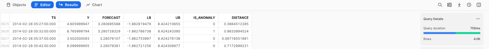
Visualizing Anomalies and Interpreting the Results
Use Snowsight to review and visualize the results of anomaly detection. In Snowsight, when you call the <model_name>!DETECT_ANOMALIES method, the results are displayed in a table under the worksheet.

To visualize the results, you can use the chart feature in Snowsight.
-
After calling the <model_name>!DETECT_ANOMALIES method, select Charts above the results table.
-
In the Data section on the right side of the chart:
- Select the Y column, and under Aggregation, select None.
- Select the TS column, and under Bucketing, select None.
-
Add the LOWER_BOUND and UPPER_BOUND columns, and under Aggregation, select None.
-
To display the initial visualization, select Chart.
-
Select Add Column on the right side of the page, and select the columns you want to visualize:
- LOWER_BOUND
- UPPER_BOUND
- IS_ANOMALY
Results:
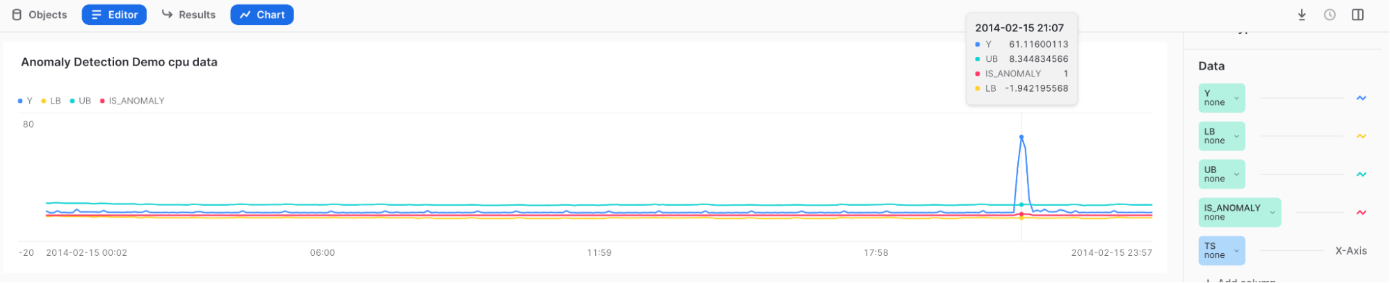
-
Hover over the high spike to see that Y lies outside of the upper bound and is tagged with a 1 in the IS_ANOMALY field.
Tip
To better understand your results, try Top Insights.
Automate Anomaly Detection with Snowflake Tasks and Alerts
You can create an automated anomaly detection pipeline, both for retraining the model and for monitoring your data for anomalies, by using Anomaly Detection functions within Snowflake Tasks or Alerts.
- Recurring Training with a Snowflake Task
- Monitoring with a Snowflake Task
- Monitoring with a Snowflake Alert
Recurring Training with a Snowflake Task
You can update your model to reflect the most up-to-date data using Snowflake Tasks.
To create a task that refreshes the anomaly detection object every hour, run following statement, replacing your_warehouse_name with your warehouse name:
By default, newly created tasks are suspended.
To resume the task, execute the ALTER TASK … RESUME command:
To pause the task, execute the ALTER TASK … SUSPEND command:
Monitoring with a Snowflake Task
You can also use Snowflake Tasks to monitor your data at a given frequency.
First, create a table to hold the results of anomaly detection:
Create a task to store the results of a recurring anomaly detection operation in the table.
This example sets the WAREHOUSE parameter to snowhouse. You can replace that with
your own warehouse:
To resume the task, execute the ALTER TASK … RESUME command:
anomaly_res_table then contains all the results for each task run.
To pause the task, execute the ALTER TASK … SUSPEND command:
Monitoring with a Snowflake Alert
You can also use Snowflake Alerts to monitor your data at a given frequency and send you email with detected anomalies. The following statements create an alert that detects anomalies every minute. First you define a stored procedure to detect anomalies, then create an alert that uses that stored procedure.
Note
You must set up email integration to send mail from a stored procedure; see Notifications in Snowflake.
To start or resume the alert, execute the ALTER ALERT … RESUME command:
To pause the alert, execute the ALTER ALERT … SUSPEND command:
Understanding Feature Importance
An anomaly detection model can explain the relative importance of all features used in your model, including any exogenous variables that you choose, automatically generated time features (such as day of week or week of year), and transformations of your target variable (such as rolling averages and auto-regressive lags). This information is useful in understanding what factors are really influencing your data.
The <model_name>!EXPLAIN_FEATURE_IMPORTANCE method counts the number of times the model’s trees used each feature to make a decision. These feature importance scores are then normalized to values between 0 and 1 so that their sum is 1. The resulting scores represent an approximate ranking of the features in your trained model.
Features that are close in score have similar importance. For extremely simple series (for example, when the target column has a constant value), all feature importance scores may be zero.
Using multiple features that are very similar to each other may result in reduced importance scores for those features. For example, if one feature is quantity of items sold and another is quantity of items in inventory, the values may be correlated because you can’t sell more than you have and because you try to manage inventory so you won’t have more in stock than you will sell. If two features are identical, the model may treat them as interchangeable when making decisions, resulting in feature importance scores that are half of what those scores would be if only one of the features were included.
Feature importance also reports lag features. During training, the model infers the frequency (hourly, daily, or weekly)
of your training data. The feature lagx (e.g. lag24) is the value of the target variable x time units ago.
For example, if your data is inferred to be hourly, lag24 represents your target variable 24 hours ago.
All other transformations of your target variable (rolling averages, etc.) are summarized as
aggregated_endogenous_features in the results table.
Limitations
- You cannot choose the technique used to calculate feature importance.
- Feature importance scores can be helpful for gaining intuition about which features are important to your model’s accuracy, but the actual values should be considered estimates.
Example
To understand the relative importance of your features to your model, train a model, and then call <model_name>!EXPLAIN_FEATURE_IMPORTANCE. In this example, you first create random data with two exogenous variables: one that is random and therefore unlikely to be very important to your model, and one that is a copy of your target and therefore likely to be more important to your model.
Execute the following statements to generate the data, train a model on it, and get the importance of the features:
Output
Because this example uses random data, do not expect your output to match this exactly.
Inspecting Training Logs
When you train multiple series with CONFIG_OBJECT => {'ON_ERROR': 'SKIP'}, individual time series models can
fail to train without the overall training process failing. To understand which time series failed and why, call
<model_instance>!SHOW_TRAINING_LOGS.
Example
Output
Cost Considerations
For details on costs for using ML functions, see Cost Considerations in the ML functions overview.