Using Window Functions¶

Rank-Related Window Functions¶

The simplest sub-category of order-sensitive functions is the rank-related function sub-category.

The simplest rank-related function is the RANK function. The rank function simply lists the rank, which is the order of a row in an ordered window of rows. The first row in the window has rank 1; the second row in the window has rank 2; etc. The example below shows the rank order of salespeople based on amount sold:

+-------------+-------------+------+
| Salesperson | Amount Sold | Rank |
|-------------+-------------+------|
| Smith       |        2000 |    1 |
| Jones       |        1500 |    2 |
| Torkelson   |        1200 |    3 |
| Dolenz      |        1100 |    4 |
+-------------+-------------+------+

Copy

The RANK function does not sort the rows; the rows must already be in order in the window before RANK is called. To put the rows in order, use the ORDER BY sub-clause of the OVER clause.

To illustrate the ORDER BY sub-clause, consider the following example: you’d like to know where your store profit ranks among branches of the store chain, i.e. whether your store ranks first, second, third, etc. Here’s an example of using an order-sensitive window function to rank each store by profitability within its city. The rows are put in descending order (highest profit first), so the most profitable store has rank 1:

SELECT city, branch_ID, net_profit,
       RANK() OVER (PARTITION BY city ORDER BY net_profit DESC) AS rank
    FROM store_sales
    ORDER BY city, rank;
+-----------+-----------+------------+------+
| CITY      | BRANCH_ID | NET_PROFIT | RANK |
|-----------+-----------+------------+------|
| Montreal  |         3 |   10000.00 |    1 |
| Montreal  |         4 |    9000.00 |    2 |
| Vancouver |         2 |   15000.00 |    1 |
| Vancouver |         1 |   10000.00 |    2 |
+-----------+-----------+------------+------+

Copy

The output of a rank-related function depends on:

• The individual row passed to the function.

• The values of the other rows in the window passed to the function.

• The order of all the rows in the window.

Snowflake provides several different rank-related functions. The names of these functions, and more details about the syntax of rank-related window functions, are in Window Functions.

Window Frame Functions¶

A window frame is a subset of the rows in a window.

A window frame function uses a window frame to calculate things such as a moving average.

Snowflake supports two types of window frames:

• Cumulative.

• Sliding.

Sliding Window Frames¶

You can picture a sliding window frame by thinking about what you see as you look out the side window of a car as the car drives parallel to a fence. If the fence posts are spaced evenly, and if the width of the window is an integer multiple of the distance between posts, then the number of fenceposts you see remains constant; however, as you drive along, “old” fenceposts move out of your view, and “new” ones move into your view, so you don’t see the same fenceposts over time, even though you see the same number of fenceposts at all times.

A sliding window frame is a fixed-width frame that “slides along” the rows in the window, showing you a different slice of the window each time. As with the car driving past the fenceposts, the window frame moves along the data, with old rows disappearing from the frame and new rows appearing, so that the width of the frame (the number of rows in the frame) is always the same.

Sliding windows are often used to calculate moving averages. A moving average is an average that is calculated based on a fixed-size interval (e.g. number of days). The average is “moving” because although the size of the interval is constant, the actual values in the interval change over time (or over some other factor) as the window slides along.

For example, stock market analysts often analyze stocks based in part on the 13-week moving average of a stock’s price. The moving average price today is the average of price at the end of today and the price at the end of each day during the most recent 13 weeks. If stocks are traded 5 days a week, and if there were no holidays in the last 13 weeks, then the moving average is the average price on each of the most recent 65 trading days (including today).

The following example shows what happens to a 13-week (91 day) moving average of a stock price on the last day of June and the first few days of July:

• On June 30th, the function returns the average price for April 1 to June 30 (inclusive).

• On July 1st, the function returns the average price for April 2 to July 1 (inclusive).

• On July 2nd, the function returns the average price for April 3 to July 2 (inclusive).

• etc.

Note

Although sliding windows are fixed-width, when a window is first applied to a new data source, the data source might not have enough data to fill the window. For example, if record-keeping started on April 1st, then from April 1st to June 29th, the sliding window would include fewer than 91 days of data. The window’s width remains constant only after the window has finished filling.

The example below uses a small (3-day) sliding window over the first 7 days in the month. This demonstrates how the window frame slides across the window, always keeping the 3 most recent values for calculating the total within the window. This illustration takes into account that at the beginning of the period, the window might not be full:

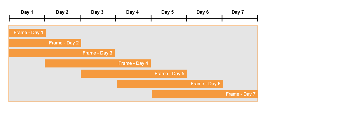
And, as you can see in the corresponding table, the last column contains the sum of the three most recent days’ worth of sales data. For example, the column value for day 4 is 36, which is the sum of the sales for days 2, 3, and 4 (11 + 12 + 13):

+--------+-------+---------------+
| Day of | Sales | Most Recent   |
| Month  | Today | 3 Days' Sales |
|--------+-------+---------------+
|      1 |    10 |            10 |
|      2 |    11 |            21 |
|      3 |    12 |            33 |
|      4 |    13 |            36 |
|      5 |    14 |            39 |
|    ... |   ... |           ... |
+--------+-------+---------------+

Copy

More Information About Order-Sensitive Window Functions¶

The PARTITION BY and ORDER BY clauses are independent. You can use the ORDER BY clause without the PARTITION BY clause. To rank your store against all other stores in the chain, not just against other stores in your city, use the query below:

SELECT
    branch_ID,
    net_profit,
    RANK() OVER (ORDER BY net_profit DESC) AS sales_rank
  FROM store_sales

SELECT
    branch_ID,
    net_profit,
    RANK() OVER (ORDER BY net_profit DESC) AS sales_rank
  FROM store_sales
  ORDER BY branch_ID;

Some window functions are order-sensitive and some are not.

• Some window functions require an ORDER BY clause.

• Some window functions prohibit an ORDER BY clause.

• Some window functions use an ORDER BY clause if one is present, but do not require it.

• Some window functions treat an ORDER BY clause as an implicit cumulative window frame clause. (More information about implied window frames is at Window Frame Usage Notes.)

The following diagram shows the relationship between window functions, window-frame functions, and rank-related functions:

                      Window Functions

  Order-insensitive Functions      Order-sensitive Functions
+-----------------------------+--------------------------------------------------------------------+
|                             | Rank-related Functions                                             |
|                             +--------------------------------------------------------------------+
|                             | Functions that can be both Rank-related and Window Frame functions |
|                             +--------------------------------------------------------------------+
|                             | Window Frame Functions                                             |
+-----------------------------+--------------------------------------------------------------------+

As shown above:

• Some window functions are not order-sensitive.

• Some window functions are order-sensitive.

• Order-sensitive window functions are divided into two categories:

  • Rank-related functions.

  • Window frame functions.

• Some order-sensitive functions are both rank-related functions and window frame functions.

Window Functions vs Aggregate Functions¶

Many window functions and aggregate functions have the same name. For example there is a SUM() window function and a SUM() aggregate function.

To distinguish between the usage of the two, remember that:

• For an aggregate function, the input is multiple rows, and the output is 1 row.

• For a window function, there are two inputs, a window of rows, and a single row inside that window, and the output is 1 row per input row.

An aggregate function tells you something, such as the SUM, about all of the rows combined, but nothing about the individual rows.

A window function tells you something about the current row relative to all the other rows in the window.

The following SQL statements show the difference between using the SUM() aggregate function, which returns 1 row for the entire group of input rows, and using the SUM() window function, which returns 1 row for each row in the group of input rows:

SELECT SUM(net_profit) 
    FROM store_sales;
+-----------------+
| SUM(NET_PROFIT) |
|-----------------|
|        44000.00 |
+-----------------+
SELECT branch_ID, SUM(net_profit) OVER ()
    FROM store_sales
    ORDER BY branch_id;
+-----------+-------------------------+
| BRANCH_ID | SUM(NET_PROFIT) OVER () |
|-----------+-------------------------|
|         1 |                44000.00 |
|         2 |                44000.00 |
|         3 |                44000.00 |
|         4 |                44000.00 |
+-----------+-------------------------+

Copy

Calculating Sales Rank¶

The Rank column is calculated using the RANK function:

SELECT day, 
       sales_today, 
       RANK()
           OVER (ORDER BY sales_today DESC) AS Rank
    FROM store_sales_2
    ORDER BY day;
+-----+-------------+------+
| DAY | SALES_TODAY | RANK |
|-----+-------------+------|
|   1 |          10 |    5 |
|   2 |          14 |    3 |
|   3 |           6 |    6 |
|   4 |           6 |    6 |
|   5 |          14 |    3 |
|   6 |          16 |    2 |
|   7 |          18 |    1 |
+-----+-------------+------+

Copy

Note that although there are 7 days in the time period, there are only 5 different ranks (1, 2, 3, 5, 6). There were two ties (for 3rd place and 6th place), so there are no rows with ranks 4 or 7.

Calculating Sales So Far This Week¶

The Sales So Far This Week column is calculated using SUM as a window function with a cumulative window frame:

SELECT day, 
       sales_today, 
       SUM(sales_today)
           OVER (ORDER BY day
               ROWS BETWEEN UNBOUNDED PRECEDING AND CURRENT ROW)
               AS "SALES SO FAR THIS WEEK"
    FROM store_sales_2
    ORDER BY day;
+-----+-------------+------------------------+
| DAY | SALES_TODAY | SALES SO FAR THIS WEEK |
|-----+-------------+------------------------|
|   1 |          10 |                     10 |
|   2 |          14 |                     24 |
|   3 |           6 |                     30 |
|   4 |           6 |                     36 |
|   5 |          14 |                     50 |
|   6 |          16 |                     66 |
|   7 |          18 |                     84 |
+-----+-------------+------------------------+

Copy

This query orders the rows by date and then, for each date, calculates the sum of sales from the start of the window up to the current date (inclusive).

Calculating Total Sales This Week¶

The Total Sales This Week column is calculated using SUM as a simple window function.

SELECT day, 
       sales_today, 
       SUM(sales_today)
           OVER ()
               AS total_sales
    FROM store_sales_2
    ORDER BY day;
+-----+-------------+-------------+
| DAY | SALES_TODAY | TOTAL_SALES |
|-----+-------------+-------------|
|   1 |          10 |          84 |
|   2 |          14 |          84 |
|   3 |           6 |          84 |
|   4 |           6 |          84 |
|   5 |          14 |          84 |
|   6 |          16 |          84 |
|   7 |          18 |          84 |
+-----+-------------+-------------+

Copy

Calculating a 3-Day Moving Average¶

The 3-Day Moving Average column is calculated using AVG as a window function with a sliding window frame:

SELECT day, 
       sales_today, 
       AVG(sales_today)
           OVER (ORDER BY day ROWS BETWEEN 2 PRECEDING AND CURRENT ROW)
               AS "3-DAY MOVING AVERAGE"
    FROM store_sales_2
    ORDER BY day;
+-----+-------------+----------------------+
| DAY | SALES_TODAY | 3-DAY MOVING AVERAGE |
|-----+-------------+----------------------|
|   1 |          10 |               10.000 |
|   2 |          14 |               12.000 |
|   3 |           6 |               10.000 |
|   4 |           6 |                8.666 |
|   5 |          14 |                8.666 |
|   6 |          16 |               12.000 |
|   7 |          18 |               16.000 |
+-----+-------------+----------------------+

Copy

The difference between this sliding window frame and the cumulative window frame described earlier is simply the starting point:

• In a sliding window frame, the starting point slides rightward.

• In a cumulative window frame, the starting point is fixed and the frame continues to accumulate with each additional row within the window.

Putting It All Together¶

Here’s the final version of our query, showing:

• Rank.

• Cumulative window frame.

• Simple window function.

• Sliding window function.

  SELECT day, 
         sales_today, 
         RANK()
             OVER (ORDER BY sales_today DESC) AS Rank,
         SUM(sales_today)
             OVER (ORDER BY day
                 ROWS BETWEEN UNBOUNDED PRECEDING AND CURRENT ROW)
                 AS "SALES SO FAR THIS WEEK",
         SUM(sales_today)
             OVER ()
                 AS total_sales,
         AVG(sales_today)
             OVER (ORDER BY day ROWS BETWEEN 2 PRECEDING AND CURRENT ROW)
                 AS "3-DAY MOVING AVERAGE"
      FROM store_sales_2
      ORDER BY day;
  +-----+-------------+------+------------------------+-------------+----------------------+
  | DAY | SALES_TODAY | RANK | SALES SO FAR THIS WEEK | TOTAL_SALES | 3-DAY MOVING AVERAGE |
  |-----+-------------+------+------------------------+-------------+----------------------|
  |   1 |          10 |    5 |                     10 |          84 |               10.000 |
  |   2 |          14 |    3 |                     24 |          84 |               12.000 |
  |   3 |           6 |    6 |                     30 |          84 |               10.000 |
  |   4 |           6 |    6 |                     36 |          84 |                8.666 |
  |   5 |          14 |    3 |                     50 |          84 |                8.666 |
  |   6 |          16 |    2 |                     66 |          84 |               12.000 |
  |   7 |          18 |    1 |                     84 |          84 |               16.000 |
  +-----+-------------+------+------------------------+-------------+----------------------+
  

  Copy

Window with PARTITION BY Clause¶

The PARTITION BY sub-clause of the windowing clause divides the data into distinct subsets based on the value of the input expression; the SELECT statement is applied to each subset, and the output has rows for each subset.

Note that this is similar to, but not identical to, how the GROUP BY clause works.

The next example shows the quantity sold each month, and uses the PARTITION BY clause to divide the data into one-month subsets:

SELECT MONTH(sales_date) AS MONTH_NUM, 
       SUM(quantity) OVER (PARTITION BY MONTH(sales_date)) AS QUANTITY
    FROM sales
    ORDER BY sales_date;
+-----------+----------+
| MONTH_NUM | QUANTITY |
|-----------+----------|
|         1 |        9 |
|         1 |        9 |
|         1 |        9 |
|         2 |        2 |
+-----------+----------+

Copy

As you can see, the first three rows are duplicates. There were 3 input rows for month #1, and the window function generates one output row for each input row, so there are 3 output rows for month #1 in the output. The SUM function is not used as a cumulative or sliding function; it is applied to the entire window and returns the same value for the entire window each time, so the function returns duplicate values as shown above.

You can reduce the duplicates by using the DISTINCT keyword:

SELECT DISTINCT MONTH(sales_date) AS MONTH_NUM, 
       SUM(quantity) OVER (PARTITION BY MONTH(sales_date))
    FROM sales
    ORDER BY MONTH_NUM;
+-----------+-----------------------------------------------------+
| MONTH_NUM | SUM(QUANTITY) OVER (PARTITION BY MONTH(SALES_DATE)) |
|-----------+-----------------------------------------------------|
|         1 |                                                   9 |
|         2 |                                                   2 |
+-----------+-----------------------------------------------------+

Copy

In this particular case, you can use a GROUP BY clause rather than a windowing clause. For example:

SELECT MONTH(sales_date) AS MONTH_NUM, 
       SUM(quantity)
    FROM sales
    GROUP BY MONTH_NUM
    ORDER BY MONTH_NUM;
+-----------+---------------+
| MONTH_NUM | SUM(QUANTITY) |
|-----------+---------------|
|         1 |             9 |
|         2 |             2 |
+-----------+---------------+

Copy

However, GROUP BY is not as flexible as windowing. Also, in more complex queries, you can’t always substitute GROUP BY for a window clause.

Window with ORDER BY Clause¶

The ORDER BY clause controls the order of the data within each window (and each partition if there is more than one partition). This is useful if you want to show a “running sum” over time as new rows are added.

A running sum can be calculated either from the beginning of the window to the current row (inclusive) or from the current row to the end of the window.

A query can use a “sliding” window, which is a fixed-width window that processes N specified rows relative to the current row (e.g. the 10 most recent rows, including the current row).

Both cumulative and sliding windows are explained below.

Window with PARTITION BY and ORDER BY Clauses¶

You can combine PARTITION BY and ORDER BY clauses to get running sums within partitions. In this example, the partitions are one month, and because the sums apply only within a partition, the sum is reset to 0 at the beginning of each new month:

SELECT MONTH(sales_date) AS MONTH_NUM,
       SUM(quantity) OVER (PARTITION BY MONTH(sales_date) ORDER BY sales_date)
          AS MONTHLY_CUMULATIVE_SUM_QUANTITY
    FROM sales
    ORDER BY sales_date;

Copy

The query result includes additional comments showing how the MONTHLY_CUMULATIVE_SUM_QUANTITY column was calculated:

+-----------+---------------------------------+
| MONTH_NUM | MONTHLY_CUMULATIVE_SUM_QUANTITY |
|-----------+---------------------------------+
|         1 |                               1 |  -- sum = 1
|         1 |                               4 |  -- sum = 1 + 3
|         1 |                               9 |  -- sum = 1 + 3 + 5
|         2 |                               2 |  -- sum = 0 + 2 (new month)
+-----------+---------------------------------+

Copy

You can combine partitions and sliding windows. In the example below, the sliding window is usually two rows wide, but each time a new partition (i.e. new month) is reached, the sliding window starts with only the first row in that partition:

SELECT
       MONTH(sales_date) AS MONTH_NUM,
       quantity,
       SUM(quantity) OVER (PARTITION BY MONTH(sales_date) 
                           ORDER BY sales_date
                           ROWS BETWEEN 1 PRECEDING AND CURRENT ROW) 
         AS MONTHLY_SLIDING_SUM_QUANTITY
    FROM sales
    ORDER BY sales_date;

Copy

The query result includes additional comments showing how the MONTHLY_SLIDING_SUM_QUANTITY column was calculated:

+-----------+----------+------------------------------+
| MONTH_NUM | QUANTITY | MONTHLY_SLIDING_SUM_QUANTITY |
|-----------+----------+------------------------------+
|         1 |        1 |                           1  |  -- sum = 1
|         1 |        3 |                           4  |  -- sum = 1 + 3
|         1 |        5 |                           8  |  -- sum = 3 + 5
|         2 |        2 |                           2  |  -- sum = 0 + 2 (new month)
+-----------+----------+------------------------------+

Copy