Snowflake interactive analytics¶

Overview¶

Snowflake interactive analytics provides low-latency, high-concurrency query execution through interactive warehouses. An interactive warehouse contains a query engine optimized for sub-second response times and high throughput, making it ideal for real-time dashboards, data-powered APIs, and high-concurrency serving workloads.

Interactive warehouses support the following table types:

Interactive tables

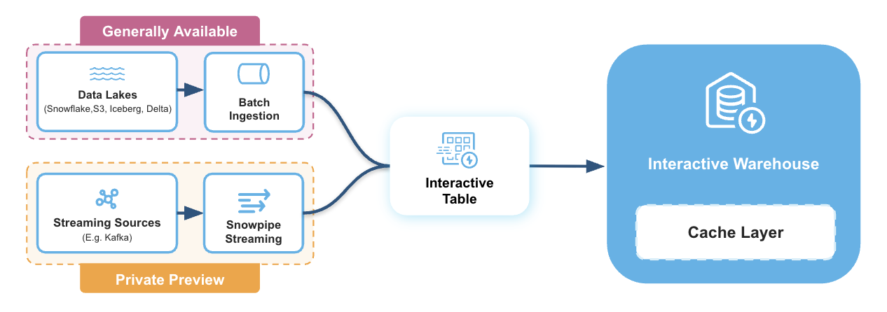
A specialized table type optimized for low-latency, high-concurrency workloads. Interactive tables require a CLUSTER BY clause and provide the best performance when queried through interactive warehouses. Interactive tables are generally available.

Standard tables and Iceberg tables (Public Preview)

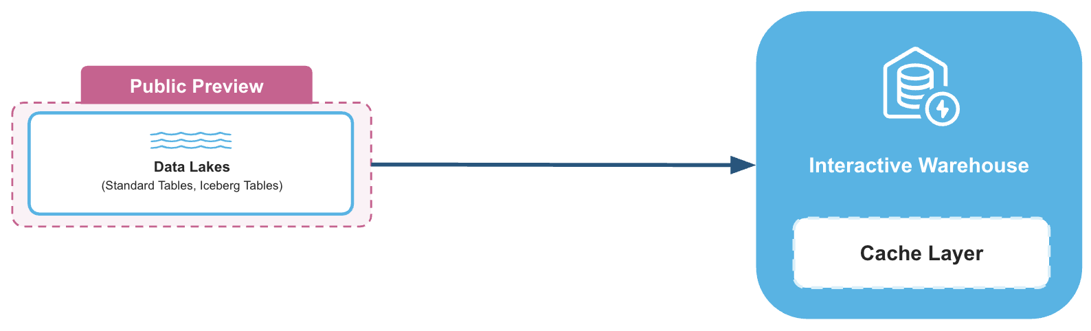
You can query standard tables and Iceberg tables directly through an interactive warehouse without copying or transforming your data. This zero-copy approach lets you benefit from the performance characteristics of interactive warehouses on your existing data.

Use cases¶

Real-time dashboards

Serving selective dashboard queries that power thousands of user requests with low-latency, high concurrency. Especially useful for serving use cases where some aggregations and flexibility are required.

Data-powered APIs

Serving data-powered APIs that require predictable, consistent latency, that contain repetitive query shapes.

Alerting and selective agentic AI workloads

For observability and selective AI agentic workloads that can generate unpredictable query load spikes and require low cost per query.

Getting started¶

To get started with interactive analytics:

1. Create an interactive warehouse. For more information, see Creating an interactive warehouse.
2. Resume the interactive warehouse. For more information, see Resuming and suspending an interactive warehouse.
3. Add tables to the interactive warehouse. For more information, see Adding tables to an interactive warehouse.
4. Start querying through the interactive warehouse. For more information, see Querying tables through an interactive warehouse.

If you want to use interactive tables for maximum performance, create the interactive table first using a standard warehouse. For more information, see Creating an interactive table.

Working with interactive warehouses¶

Creating an interactive warehouse¶

Specify the keyword INTERACTIVE in the CREATE WAREHOUSE or CREATE OR REPLACE WAREHOUSE command.

Optionally, you can specify a TABLES clause with a comma-separated list of table names. Using that clause immediately associates those tables with the interactive warehouse.

The following command creates an interactive warehouse associated with a table named orders. You can immediately run a USE WAREHOUSE command for the interactive warehouse and begin running queries:

CREATE OR REPLACE INTERACTIVE WAREHOUSE interactive_demo
  TABLES (orders)
  WAREHOUSE_SIZE = 'XSMALL';

The following command creates an interactive warehouse with no associated tables. You can run ALTER WAREHOUSE commands afterward to associate tables with the interactive warehouse:

CREATE OR REPLACE INTERACTIVE WAREHOUSE interactive_demo
  WAREHOUSE_SIZE = 'XSMALL';

After you create an interactive warehouse, it remains in a suspended state until you resume it. You can configure auto-suspend and auto-resume for interactive warehouses. The minimum auto-suspend interval for an interactive warehouse is 24 hours (86400 seconds). For details, see Resuming and suspending an interactive warehouse.

Resuming and suspending an interactive warehouse¶

The following command resumes an interactive warehouse.

ALTER WAREHOUSE interactive_demo RESUME;

You also do this to start running queries through the warehouse, if you manually suspended the warehouse.

Queries will be slow while the cache is being warmed after resuming. Warming speed is based on the size of the data and the warehouse size. A XS warehouse warms roughly at 300-400MB/s. The bigger the table, the longer the cache warming time. Larger warehouses warm faster.

The following command suspends an interactive warehouse:

ALTER WAREHOUSE interactive_demo SUSPEND;

Auto-suspend and auto-resume for interactive warehouses¶

Interactive warehouses support auto-suspend and auto-resume. You can set the AUTO_SUSPEND and AUTO_RESUME properties when creating or altering an interactive warehouse.

The minimum AUTO_SUSPEND value for an interactive warehouse is 86400 seconds (24 hours). This minimum ensures that the cache stays warm long enough to provide consistent low-latency performance. AUTO_SUSPEND will be set to 86400 if you specify a value less than 86400.

The following example creates an interactive warehouse with auto-suspend after 24 hours of inactivity, and auto-resume enabled:

CREATE INTERACTIVE WAREHOUSE interactive_demo
  WAREHOUSE_SIZE = 'XSMALL'
  AUTO_SUSPEND = 86400
  AUTO_RESUME = TRUE;

You can also set these properties on an existing interactive warehouse:

ALTER WAREHOUSE interactive_demo SET
  AUTO_SUSPEND = 86400
  AUTO_RESUME = TRUE;

Adding tables to an interactive warehouse¶

Adding a table to an interactive warehouse indicates to Snowflake that this table should be maintained in the data cache. You can add interactive tables, standard tables, and Iceberg tables.

If you didn’t specify tables to associate with the interactive warehouse by using the TABLES clause in your CREATE INTERACTIVE WAREHOUSE command, you can do that later by using an ALTER WAREHOUSE command.

To run this command, the role must have the MANAGE ATTACHED TABLES or MODIFY privilege on the warehouse. Use MANAGE ATTACHED TABLES to grant scoped access to cache management operations without granting full warehouse modification rights:

GRANT MANAGE ATTACHED TABLES ON WAREHOUSE interactive_demo TO ROLE data_engineer;

The following command associates the orders table with the interactive_demo warehouse. You can specify multiple table names, separated by commas, with the ADD TABLES clause.

ALTER WAREHOUSE interactive_demo ADD TABLES (orders);

If the table is already associated with the interactive warehouse, the command succeeds but has no effect. You can associate a table with multiple interactive warehouses.

This action starts the data cache-warming process. Cache warming time is based on the size of the data and the warehouse size. A XS warehouse warms roughly at 300-400MB/s. The bigger the table, the longer the cache warming time. Larger warehouses warm faster.

The warming process doesn’t block the warehouse from accepting new queries. Priority of warming is:

1. User issued queries
2. Newly added micropartitions through auto-refresh or other means of data ingestion
3. Any existing data

We strongly recommend adding tables you use frequently to your interactive warehouse. This helps you achieve lower latency and higher concurrency.

Because cache warming depends on your queries, the best way to monitor whether the cache is warm is to review the remote read percentage in Snowsight Query Profile. For programmatic access to query operator statistics, see GET_QUERY_OPERATOR_STATS. In ideal execution scenarios, low-latency queries should have a remote read percentage of 0%.

Querying tables through an interactive warehouse¶

In your query session, ensure that the warehouse for your current session is an interactive warehouse:

USE WAREHOUSE interactive_demo;

After this, you can query your tables normally. Interactive warehouses support interactive tables, standard tables, and Iceberg tables. Hybrid tables aren’t supported.

Removing tables from an interactive warehouse¶

You can detach one or more tables from an interactive warehouse by running an ALTER WAREHOUSE command with the DROP TABLES clause. To run this command, the role must have the MANAGE ATTACHED TABLES or MODIFY privilege on the warehouse.

ALTER WAREHOUSE interactive_demo DROP TABLES (orders, customers);

Automatically handling statement timeouts¶

To optimize for high concurrency queries on interactive warehouses, Snowflake automatically cancels queries after 5 seconds. You have an option to specify a fallback warehouse to allow automatic re-run of timed-out queries. By offloading timed-out queries to a secondary compute resource, you ensure that temporary resource contention or large scans don’t block the interactive user experience.

This fallback behavior is transparent to the client issuing the query, it behaves as an internal retry mechanism.

Configuring a fallback warehouse provides an automated retry mechanism for these canceled queries that exceed 5 seconds. When a fallback warehouse is added to an interactive warehouse, any query that exceeds the timeout threshold on the primary warehouse is automatically cancelled and retried on the designated fallback warehouse.

• Timeout Threshold: The STATEMENT_TIMEOUT_IN_SECONDS for queries on Interactive Warehouses are fixed at a default and maximum of 5 seconds. If a query doesn’t complete within this window, then Snowflake automatically retries the query on the fallback warehouse.
• Retry Logic: When a retry on fallback warehouse occurs, the failed query time shows up in fault_handling_time in query profile.
• Warehouse State: The fallback warehouse must be started (or set to auto-resume) to accept the retried query. Standard credit consumption applies to the fallback warehouse once it is active.
• RBAC requirements: To query with fallback support, the querying role must have USAGE on both the interactive warehouse and its fallback warehouse. To set a fallback warehouse, the administrator role must have ALTER WAREHOUSE on the interactive warehouse and USAGE on the fallback warehouse.

To set a fallback warehouse, you can use the following command:

ALTER WAREHOUSE interactive_demo SET FALLBACK_WAREHOUSE = <fallback_warehouse_name>;

To remove a fallback warehouse, you can use the following command:

ALTER WAREHOUSE interactive_demo UNSET FALLBACK_WAREHOUSE;

To view the fallback warehouse for an interactive warehouse, you can use the following command:

SHOW WAREHOUSES like '%interactive_demo%';

and inspect the FALLBACK_WAREHOUSE column.

Auto-scaling for high-concurrency¶

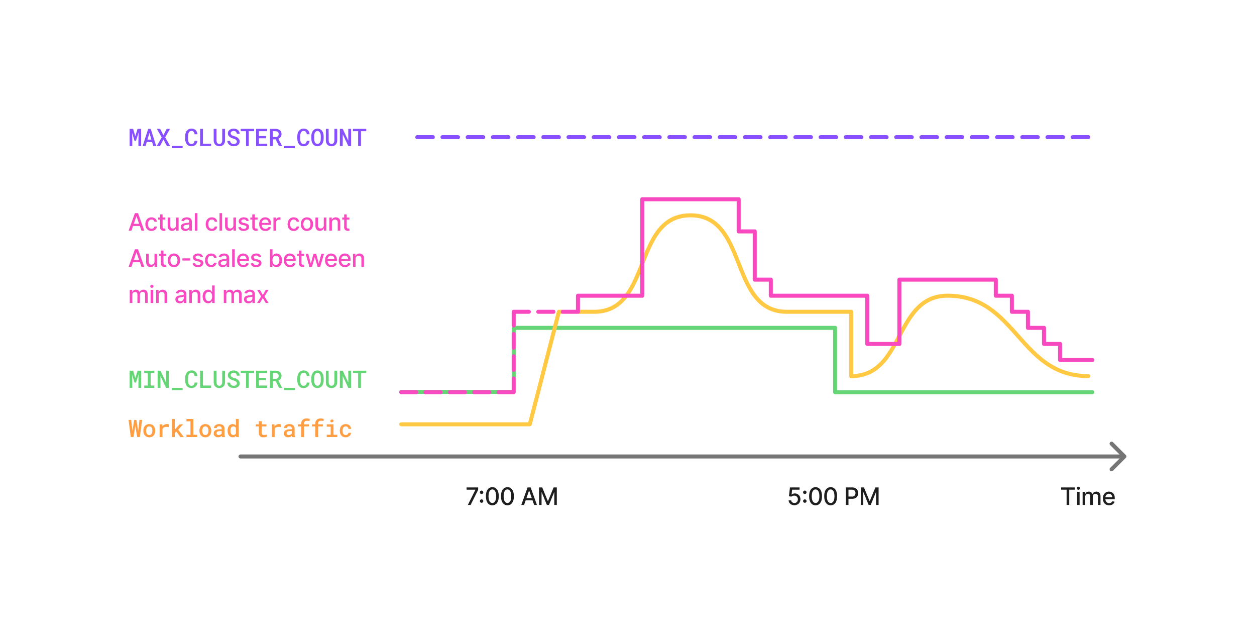
For workloads that require high-concurrency, that is, high queries per second, set the MAX_CLUSTER_COUNT using auto-scaling policy to accommodate peak concurrency for your workload and MIN_CLUSTER_COUNT to accommodate base concurrency. Typically, we recommend using scheduled scaling to configure MIN_CLUSTER_COUNT to warm up warehouses before workload surges, and using MAX_CLUSTER_COUNT to handle unpredictable spikes in concurrency.

-- 1) Task to scale OUT during business hours
CREATE OR REPLACE TASK mcw_scale_out_morning
  WAREHOUSE = my_wh          -- the warehouse that *executes the task*
  SCHEDULE = 'USING CRON 11 8 * * * UTC'   -- 08:11 UTC daily; use a random minute such as 11
AS
  ALTER WAREHOUSE my_wh      -- the warehouse you want to change (can be same or different)
    SET
      MIN_CLUSTER_COUNT = 10;  -- optional: ECONOMY or STANDARD

-- 2) Task to scale IN after hours
CREATE OR REPLACE TASK mcw_scale_in_evening
  WAREHOUSE = my_wh
  SCHEDULE = 'USING CRON 2 20 * * * UTC'  -- 20:02 UTC daily; use a random minute such as 2
AS
  ALTER WAREHOUSE my_wh
    SET
      MIN_CLUSTER_COUNT = 2;

Dropping an interactive warehouse¶

You can run the DROP WAREHOUSE command to remove an interactive warehouse entirely. Dropping an interactive warehouse removes the associations between that warehouse and any tables. However, you can still use other interactive warehouses to query those same tables.

Working with interactive tables¶

Interactive tables are a specialized table type designed for maximum performance with interactive warehouses. They require a CLUSTER BY clause and support auto-refresh from a source table.

Creating an interactive table¶

Table creation follows the standard CTAS (CREATE TABLE AS SELECT) syntax, with the additional INTERACTIVE keyword that defines the table type.

The CREATE INTERACTIVE TABLE command also requires a CLUSTER BY clause. Specify one or more columns in the CLUSTER BY clause to match the WHERE clauses in your most time-critical queries. The columns you specify in the CLUSTER BY clause can significantly affect the performance of queries on the interactive table. Therefore, choose the clustering columns carefully. For more information about choosing the best clustering columns, see Clustering Keys & Clustered Tables.

The following command creates an interactive table containing the same columns and data as a standard table. The CLUSTER BY clause refers to a column named id from the source table.

CREATE INTERACTIVE TABLE
  IF NOT EXISTS orders
  CLUSTER BY (id)
AS
  SELECT * FROM demoSource;

Specifying auto-refresh for an interactive table¶

To make an interactive table automatically refresh using data from some other table, specify the TARGET_LAG clause with an interval. When you specify TARGET_LAG, you must also specify the WAREHOUSE clause and the name of a standard warehouse that Snowflake will use for regular maintenance refreshes.

You can also optionally specify INITIALIZATION_WAREHOUSE to run initial refreshes on a separate warehouse. Initial refreshes often process more data than maintenance refreshes. In many cases, you can use a larger warehouse, such as 2XL, for the initial refresh and a smaller warehouse, such as S, for ongoing maintenance refreshes.

The time interval for the TARGET_LAG clause lets you specify the maximum lag in terms of some number of minutes, hours, or days:

TARGET_LAG = '<num> { seconds | minutes | hours | days }'

If you don’t specify a unit, the number represents seconds. The minimum value is 60 seconds, or 1 minute.

For example, the following CREATE INTERACTIVE TABLE statement defines an interactive table that lags no more than 20 minutes behind a specified source table, uses a larger warehouse for the initial refresh, and uses a smaller warehouse for ongoing maintenance refreshes:

CREATE INTERACTIVE TABLE my_dynamic_interactive_table
  CLUSTER BY (c1, c2)
  TARGET_LAG = '20 minutes'
  WAREHOUSE = s_maintenance_wh
  INITIALIZATION_WAREHOUSE = xl_initial_wh
AS SELECT c1, SUM(c2) FROM my_source_table GROUP BY c1;

For more information about choosing an appropriate lag time that balances costs and freshness of data, see How Snowflake uses target lag. For guidance on using separate warehouses for initial and maintenance refreshes, see WAREHOUSE vs INITIALIZATION_WAREHOUSE. Similar considerations apply to interactive tables as to dynamic tables.

You can also manually trigger a refresh for a dynamic interactive table by running

ALTER INTERACTIVE TABLE ``my_dynamic_interactive_table`` REFRESH.

Materialized view support for interactive tables¶

You can create materialized views on interactive tables. An interactive materialized view precomputes and stores the results of a query on an interactive table, which can further improve query performance for common aggregation patterns.

To create an interactive materialized view, use the INTERACTIVE keyword in the CREATE MATERIALIZED VIEW statement:

CREATE INTERACTIVE MATERIALIZED VIEW IF NOT EXISTS mv_order_summary
  AS
    SELECT region, SUM(quantity) AS total_quantity, SUM(net_paid) AS total_net_paid
      FROM orders
      GROUP BY region;

After you create the interactive materialized view, you must add both the materialized view and the underlying base table to your interactive warehouse:

ALTER WAREHOUSE interactive_demo ADD TABLES (mv_order_summary, orders);

Best practices for interactive materialized views¶

Follow these guidelines when you create materialized views using interactive tables:

• Interactive materialized views work just like regular materialized views. It must be based on an interactive table.
• The interactive materialized view and the source interactive table it is based on must be added to the same interactive warehouse.
• Joins aren’t supported in materialized views, whether interactive or standard. Structure your queries to aggregate or filter from a single base table.
• You can’t use an interactive table or an interactive materialized view as the source for a dynamic table.
• When you’re considering candidates for interactive materialized views, choose aggregation queries that are frequently run and expensive to compute.

Interactive tables and storage lifecycle policies¶

You can use storage lifecycle policies to archive or expire specific table rows based on conditions that you define, such as data age or other criteria.

Currently, you can’t use storage lifecycle policies for interactive tables that use auto-refresh. You can use the TARGET_LAG parameter, or a storage lifecycle policy, but not both.

Limitations of interactive tables¶

• Interactive tables don’t support the following features:

  • Data manipulation language (DML) commands such as UPDATE and DELETE. The recommended workflow is to use auto-refresh interactive tables (by setting TARGET_LAG) and apply DML to the source table instead. The auto-refresh mechanism is more efficient and cost-effective than using DML on the interactive table. The only DML that you can perform is INSERT OVERWRITE.
  • Fail-safe. This data recovery mechanism isn’t available for interactive tables. However, you can still use Time Travel with interactive tables.
  • Query insights. They currently aren’t collected or available for queries executing on interactive tables to help reduce query execution latency when queries are executed using SDKs. Snowsight queries still produce insights, but at a cost of higher query latency.

• You can’t perform the following operations:

  • Use an interactive table as the source for a standard (non-interactive) materialized view. To create a materialized view on an interactive table, use the INTERACTIVE keyword. See Materialized view support for interactive tables.

  • Modify properties of an interactive table by using ALTER TABLE clauses such as ADD COLUMN or REMOVE COLUMN. ALTER TABLE operations that you can perform include:

    • Renaming the table.
    • Modifying columns to set or unset comments.
    • Setting or unsetting masking policies on columns.
    • Adding or unsetting a masking policy, join policy, aggregation policy, or row access policy on the table.
    • Adding a storage lifecycle policy to the table, or dropping a storage lifecycle policy from the table.

  • Use streams with an interactive table.

  • Create a dynamic table with an interactive table as a base table.

  • Use the RESAMPLE clause for queries on an interactive table.

  • Set the Time Travel retention period using CREATE INTERACTIVE TABLE or ALTER TABLE. Interactive tables inherit the DATA_RETENTION_TIME_IN_DAYS value from their parent schema, database, or account.

Using standard and Iceberg tables (Public Preview)¶

You can use interactive warehouses to query standard tables and Iceberg tables directly, without copying or transforming your data into interactive tables. This zero-copy approach lets you benefit from the performance characteristics of interactive warehouses on your existing data.

Interactive warehouses limit query run time to 5 seconds; after 5 seconds, the warehouse can transparently fall back to a fallback standard warehouse of your choice to protect the timing of the next query. For more information about fallback warehouses, see Automatically handling statement timeouts.

Getting started with standard and Iceberg tables¶

To use an interactive warehouse with a standard table or an Iceberg table, create the interactive warehouse, set it as the active warehouse, and then query your tables as you would with a standard warehouse.

Standard and Iceberg tables can be attached to an interactive warehouse the same way you attach interactive tables, using ALTER WAREHOUSE … ADD TABLES. For more information, see Adding tables to an interactive warehouse.

Example: querying standard tables with an interactive warehouse¶

Start by creating a database to work with TPC-H data.

CREATE DATABASE demo;
USE DATABASE demo;

Then move data from the sample database into this newly created database so that you can experiment freely.

CREATE OR REPLACE WAREHOUSE standard_demo WAREHOUSE_SIZE = 'XLARGE';

USE WAREHOUSE standard_demo;

CREATE OR REPLACE TABLE LINEITEM
  CLUSTER BY (L_SHIPDATE, L_ORDERKEY)
  AS SELECT * FROM SNOWFLAKE_SAMPLE_DATA.TPCH_SF100.LINEITEM;

CREATE OR REPLACE TABLE ORDERS
  CLUSTER BY (O_ORDERDATE, O_ORDERKEY)
  AS SELECT * FROM SNOWFLAKE_SAMPLE_DATA.TPCH_SF100.ORDERS;

CREATE OR REPLACE TABLE CUSTOMER
  CLUSTER BY (C_MKTSEGMENT, C_NATIONKEY)
  AS SELECT * FROM SNOWFLAKE_SAMPLE_DATA.TPCH_SF100.CUSTOMER;

CREATE OR REPLACE TABLE PART
  CLUSTER BY (P_BRAND, P_SIZE)
  AS SELECT * FROM SNOWFLAKE_SAMPLE_DATA.TPCH_SF100.PART;

CREATE OR REPLACE TABLE PARTSUPP
  CLUSTER BY (PS_PARTKEY, PS_SUPPKEY)
  AS SELECT * FROM SNOWFLAKE_SAMPLE_DATA.TPCH_SF100.PARTSUPP;

CREATE OR REPLACE TABLE SUPPLIER
  CLUSTER BY (S_NATIONKEY)
  AS SELECT * FROM SNOWFLAKE_SAMPLE_DATA.TPCH_SF100.SUPPLIER;

CREATE OR REPLACE TABLE NATION
  AS SELECT * FROM SNOWFLAKE_SAMPLE_DATA.TPCH_SF100.NATION;

CREATE OR REPLACE TABLE "REGION"
  AS SELECT * FROM SNOWFLAKE_SAMPLE_DATA.TPCH_SF100.REGION;

ALTER WAREHOUSE standard_demo SET WAREHOUSE_SIZE = 'XSMALL';

SHOW TABLES;

Now create an interactive warehouse. Because the copied TPC-H dataset is only 100 GB, the XSMALL size is more than enough to start. You can attach the created tables to the interactive warehouse to let Snowflake know that these tables should be moved into the interactive warehouse cache right away.

CREATE OR REPLACE INTERACTIVE WAREHOUSE interactive_demo WAREHOUSE_SIZE = 'XSMALL';

ALTER WAREHOUSE interactive_demo
ADD TABLES (LINEITEM, ORDERS, CUSTOMER, PART, PARTSUPP, SUPPLIER);

USE WAREHOUSE interactive_demo;

As you can see from the code above, the tables NATION and REGION, just as an example, haven’t been attached to the created interactive warehouse. They can still be queried using an interactive warehouse and their content will be moved into the interactive warehouse cache as needed.

Note that clustering is not strictly needed for using tables with an Interactive Warehouse. However, for better performance it is highly recommended, as it helps significantly with partition pruning.

Now you can run a query on the tables you created. Run the query a few times to see real performance. If you just created the interactive warehouse, data might not be in cache on the first run.

SELECT
    N_NAME,
    COUNT(*) AS ORDERS
FROM
    ORDERS AS O
INNER JOIN
    CUSTOMER AS C ON O_CUSTKEY = C_CUSTKEY
INNER JOIN
    NATION AS N ON C_NATIONKEY = N_NATIONKEY
WHERE
    O_ORDERDATE BETWEEN '1996-01-1' AND '1996-12-31'
GROUP BY ROLLUP
    (N_NAME)
ORDER BY
    N_NAME NULLS LAST
;

The above query is well suited for interactive workloads because it has all the characteristics of an interactive query:

• It is selective enough.
• It takes advantage of the clustering key.
• It returns a few rows.

Known issues for standard and Iceberg tables¶

Performance of interactive warehouses on Iceberg tables may be lower than performance on standard tables during this preview.

Performance considerations¶

• Query best practices for interactive warehouses
• Data layout best practices
• Choosing a size for an interactive warehouse
• Performance optimization for interactive analytics
• Using search optimization for point lookups

The following sections explain how to solve performance issues that you might encounter due to the special characteristics of interactive warehouses and the workloads they’re best suited for.

Query best practices for interactive warehouses¶

Interactive warehouses are optimized for queries with selective workloads. This means queries with good selectivity see substantially more improvements on performance than other query types.

Scenario 1: Narrow projection versus full-table projection¶

This query is likely to see more benefit:

SELECT col1, col4, AVG(col_x)
  FROM my_table
  GROUP BY col1, col4;

This query is highly selective because it only requires a few columns. Snowflake can optimize loading only columns required for this one query.

This query is likely to see limited benefit:

SELECT * FROM my_table;

This query processes all columns. Although the query is simple, Snowflake must process a large amount of data, which might exceed the size of the cache. Even if the content of the table can fit in the cache, causing other queries to load new data into the cache at runtime, leading to lower concurrency.

Scenario 2: Targeted filters versus broad time-range filters¶

This query is likely to see more benefit:

SELECT col1, col2
  FROM my_table
  WHERE
    col_x IN (1,4,7,8)
    AND event_time >=
      DATEADD(hour, -1, CURRENT_TIMESTAMP());

The conditions in the WHERE clause make this query highly selective. The IN clause limits the results to a relatively few items, and the time comparison further limits the data to a certain time period.

This query is likely to see limited benefit:

SELECT col1, col2
  FROM my_table
  WHERE
    event_time >=
      DATEADD(day, -365, CURRENT_TIMESTAMP());

Asking for data for an entire year makes this query less selective. If your dataset is big, this query might process all rows in the table.

Other complexities such as large joins (for example, by joining two fact tables), or compute-intensive expressions such as regular expressions, might result in lower concurrency due to higher use of compute resources. See Choosing a size for an interactive warehouse for information about optimizing for those situations.

Data layout best practices¶

Tables queried through interactive warehouses benefit from a well-clustered table, a table that’s sorted based on the same column or columns that you are filtering on. For example, if your query often filters on a TIMESTAMP column such as sale_date, then it makes sense to use that column as the clustering key.

For interactive tables, you specify the clustering key during creation:

CREATE INTERACTIVE TABLE product_sales (<column definitions>) CLUSTER BY (sale_date);

For standard tables, use the ALTER TABLE … CLUSTER BY command to set or change the clustering key.

That way, SELECT queries that filter on sale_date can quickly skip all irrelevant data and return results. For example, the following query filters on a date range by testing the sale_date column:

SELECT ... WHERE sale_date > '2025-10-24' AND ...

For more details about choosing the best clustering keys, see Clustering Keys & Clustered Tables.

Interactive tables support up to 1 KB total across all clustering key columns. The per-column 5-byte limit for standard tables doesn’t apply.

Snowflake Cortex Code supports automatic clustering key selection for interactive tables. To use it, start Cortex Code and prompt it to suggest a clustering key using the interactive-clustering-key-recommendation skill.

Choosing a size for an interactive warehouse¶

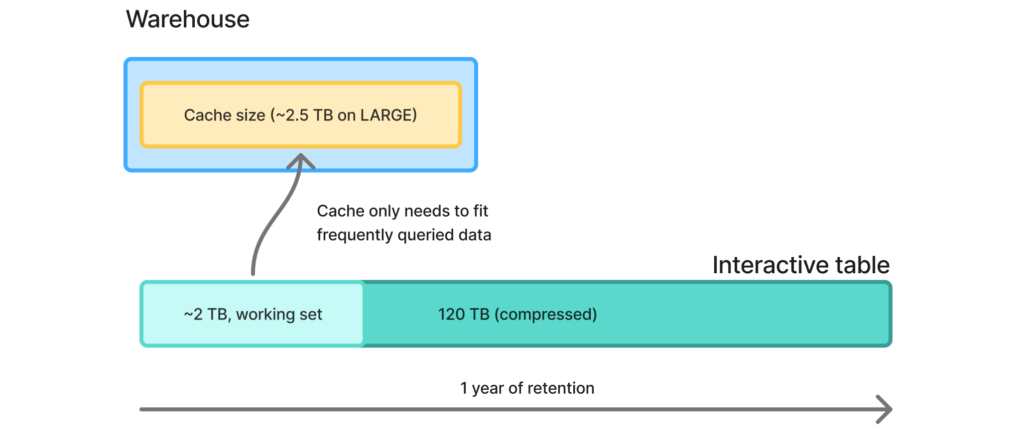
You should start by sizing your warehouse based on the approximate size of the working set in your tables. Interactive warehouses pre-warm the data cache based on tables you’ve attached to the warehouse via ALTER WAREHOUSE ADD TABLES(table_1, table_2, …).

For example, if your table is 120TB (compressed), and it represents 1 year worth of data. If you mostly query the last 7 days, then you should size your warehouse as MEDIUM to be able to hold the last 7 days of data. (120TB / 365 days * 7 days = 2.19TB) Interactive warehouses have a range of sizes from XSMALL to 4XLARGE, see the warehouse sizing table for more information.

Once you’ve completed all your queries and layout optimizations, consider scaling your warehouse to meet demand. Choose a minimum number of clusters sufficient to support the expected number of concurrent users, see Multi-cluster warehouses.

This is because the interactive warehouse utilizes local storage caching. While the data for your entire data set (table) is always accessible, accessing non-cached data does incur higher read latency on the first read.

Choose a warehouse size to fit the needs of your workloads. Experiment with your data and workload to determine the optimal size for your interactive warehouse.

Performance optimization for interactive analytics¶

Interactive analytics is optimized for short-running queries and enforces a default statement timeout of 5s. You might encounter patterns where queries run slower than expected. The following sections describe common problems, how to recognize them, and what to try.

For all of these patterns, your primary diagnostic tool is the Snowsight Query Profile, especially the remote read percentage and the time breakdown between compilation, queuing, and execution. For programmatic access to query operator statistics, see GET_QUERY_OPERATOR_STATS.

Problem 1: A single query is taking too long¶

Likely causes:

• The query needs more compute resources than the warehouse provides. Examples include predicates with regular expressions or CASE expressions, and high-memory operations like COUNT(DISTINCT ...).
• The warehouse is too small to hold a useful working set in the local data cache, so the query reads heavily from remote storage. You can see this in Query Profile as a high remote read percentage.
• The query scans more data than necessary because the ORDER BY, LIMIT, or WHERE clauses aren’t aligned with the table’s clustering keys, so micropartition pruning isn’t effective.

What to try:

• Increase the warehouse size. Start with the recommended size for your working set (see the sizing table above) and keep increasing until single-query latency is acceptable.
• Select only the columns you need, and add selective predicates in the WHERE clause so the query can effectively prune micropartitions.
• For ORDER BY + LIMIT queries (for example, “most recent N rows”), make sure the clustering key matches the column used in ORDER BY. A table clustered by its timestamp column prunes efficiently for “most recent” queries; one that isn’t clustered by the sort column might read the full table. For help choosing clustering keys, see Cortex Code clustering key recommendation.

Problem 2: Queries are suddenly taking longer (high tail latency, high P95 latency)¶

In Query Profile, the slow queries show an elevated remote read percentage compared to earlier fast queries in the same session.

Likely causes:

• The warehouse was suspended between bursts and resumed for this burst. Cache warming hasn’t finished when the first queries arrive.
• The new burst touches different micro partitions of the table than the prior workload, so the first queries read from remote storage until the new micro partitions are cached.
• The total size of all tables attached to the warehouse far exceeds the data cache capacity, so different query patterns keep evicting each other’s cached data. In this case you see chronic high remote reads across all queries, not just the first few in a burst.
• The first one or two queries immediately after a resume can show uneven per-worker latency as different nodes finish warming at slightly different times. This is typically self-resolving after a few queries.

What to try:

• If chronic high remote reads persist across all queries (not only the first few in a burst), your attached table footprint probably exceeds the data cache capacity of the warehouse. Detach unused tables with ALTER WAREHOUSE ... DROP TABLES, or use a larger warehouse size.
• For benchmarks, wait for cache warming to finish before measuring latency. Cache warm-up speed depends on warehouse size and table size: bigger tables take longer, bigger warehouses warm faster.

Problem 3: The first query of a new shape is slow, later similar queries are fast¶

In Query Profile, the slow first query spends most of its time in compilation, and later queries of the same shape compile quickly.

Likely cause:

• Query metadata caches on the compilation cache are cold for this query pattern.

What to try:

• Use bind variables instead of embedding literal values directly in SQL text. Queries that differ only in their literal values (for example, different filter parameters from a dashboard) share the same query shape, so they all benefit from a single warm compilation cache entry.
• Remember that steady production query volume keeps these caches warm. Latency measured at very low throughput does not reflect what you’ll see at realistic load.

Problem 4: Queries are queuing or you’re not achieving the expected concurrency¶

In Query Profile, queued queries spend a significant portion of their time queuing before execution starts.

Likely causes:

• The peak of concurrent queries exceeds the warehouse’s concurrency capacity.

What to try:

• Scale out by setting MIN_CLUSTER_COUNT and MAX_CLUSTER_COUNT to run a multi-cluster interactive warehouse. If MAX_CLUSTER_COUNT is greater than MIN_CLUSTER_COUNT, Snowflake adds clusters automatically as load increases.
• If your workload has a predictable ramp-up (for example, at the start of a business day), use task based multi-cluster sizing to scale out the warehouse.

Using search optimization for point lookups¶

We recommend adding search optimization when you perform point lookup queries on your tables. Point lookups are queries that filter on a single column to retrieve one or a few rows of data. A good example is WHERE some_id = some_UUID.

Benchmarking best practices¶

When assessing the performance of interactive warehouses in a test environment, follow these best practices to avoid inconsistent or misleading results:

• Turn off the query result cache to make the benchmark results consistent between multiple benchmark runs. You can turn off the query result cache at the account, user, and session level by setting the USE_CACHED_RESULT session parameter. That way, the queries only use the table data cache from the interactive warehouse. When you turn result caching on in your production environment, you can expect equal or better performance than in your benchmark testing.
• Because an interactive warehouse takes some time to warm the table data cache, wait for a while after you create or resume an interactive warehouse before testing query performance. This simulates the typical production configuration, where the warehouse remains active for long periods. Snowflake applies optimizations to the cache warming process. Therefore, it’s more efficient to let Snowflake complete this process than to warm the cache yourself by running sample queries.
• When comparing performance of interactive tables against standard Snowflake tables, don’t interleave the queries between standard and interactive tables. Instead, run the full benchmark on standard tables, then run the same tests on interactive tables.
• When doing comparative benchmarks with other database systems, make sure that the clustering columns in your tables match the WHERE clause predicates in your queries. For more information about choosing the best clustering columns, see Clustering Keys & Clustered Tables. In particular, don’t cluster on columns with high cardinality, such as unique IDs or timestamps.
• If your queries are short and simple, you can achieve higher concurrency by setting the MAX_CONCURRENCY_LEVEL parameter to a higher value for your interactive warehouse.

AI-assisted optimization with Cortex Code¶

Cortex Code includes a built-in snowflake-interactive skill that can analyze your queries and recommend how to configure interactive analytics for your workload. The skill helps you with clustering key selection, warehouse sizing, table attachment, and overall performance tuning.

To use the skill, start Cortex Code (CLI or Desktop) and describe your workload. For example:

I have the following query:

SELECT
  N_NAME,
  COUNT(*) AS ORDERS
FROM ORDERS AS O
INNER JOIN CUSTOMER AS C ON O_CUSTKEY = C_CUSTKEY
INNER JOIN NATION   AS N ON C_NATIONKEY = N_NATIONKEY
WHERE O_ORDERDATE BETWEEN '1996-01-01' AND '1996-12-31'
GROUP BY ROLLUP (N_NAME)
ORDER BY N_NAME NULLS LAST;

I want to understand how it can benefit from interactive analytics. The query
is used in a dashboard along with other queries. The query must answer in less
than a second. The database with the tables used by the query is
DM_TESTTPCH_BENCH_DB and the schema is TPCH_SF100. The filter on order date
will be different, and users might also filter data for a specific nation,
region, or market. How can I make sure that I can obtain the performance I need?
Use the "PM" connection to connect to Snowflake.

The skill connects to your Snowflake account, inspects the tables and their current clustering, evaluates the query profile, and provides recommendations including:

• Whether an interactive warehouse or interactive table is the best fit for your workload.
• Clustering key suggestions based on your filter patterns and join columns.
• Warehouse sizing guidance based on your data volume.
• Materialized view candidates for frequently run aggregation patterns.

Region availability¶

Interactive tables and interactive warehouses are available in the following Amazon Web Services (AWS), Google Cloud Platform (GCP), and Microsoft Azure regions. For more information about Snowflake regions, see Supported cloud regions.

• us-east-1 - AWS US East (N. Virginia)
• us-west-2 - AWS US West (Oregon)
• us-east-2 - AWS US East (Ohio)
• ca-central-1 - AWS Canada (Central)
• sa-east-1 - AWS South America (São Paulo)
• af-south-1 - AWS Africa (Cape Town)
• ap-northeast-1 - AWS Asia Pacific (Tokyo)
• ap-northeast-2 - AWS Asia Pacific (Seoul)
• ap-northeast-3 - AWS Asia Pacific (Osaka)
• ap-south-1 - AWS Asia Pacific (Mumbai)
• ap-southeast-1 - AWS Asia Pacific (Singapore)
• ap-southeast-2 - AWS Asia Pacific (Sydney)
• eu-central-1 - AWS EU (Frankfurt)
• eu-north-1 - AWS EU (Stockholm)
• eu-west-1 - AWS EU (Ireland)
• eu-west-2 - AWS Europe (London)
• eu-west-3 - AWS Europe (Paris)
• us-central1 - GCP US Central1 (Iowa)
• us-east4 - GCP US East4 (N. Virginia)
• europe-west2 - GCP Europe West2 (London)
• europe-west3 - GCP Europe West3 (Frankfurt)
• europe-west4 - GCP Europe West4 (Netherlands)
• australia-southeast2 - GCP Australia Southeast2 (Melbourne)
• Azure: all Azure regions.

Disaster recovery and replication¶

When added to a replication group, interactive tables and warehouses are replicated to the target account. Interactive table replication behaves the same as standard table replication.

Interactive warehouse replication assumes interactive warehouse support in the target region. Snowflake doesn’t validate interactive warehouse replication in the target region at this time. When using interactive warehouses and replication you must ensure that target region supports interactive warehouses.

The interactive warehouse in the target account will auto-resume upon querying. However, due to cache warming requirements, the performance of the warehouse is not guaranteed. To ensure consistent performance, you must keep the warehouse running in the target region.

Cost and billing considerations¶

Interactive warehouses incur compute charges when active. The minimum billable period for an interactive warehouse is one hour, and at one-second granularity thereafter.

Interactive tables incur standard storage costs. The price for storage of interactive tables is the same as for standard tables per TB. Interactive tables might be larger than equivalent standard tables, due to differences in data encoding and additional indexes. The larger data size and indexes are factored into the storage volume.

For more information about cost and billing for interactive warehouses and interactive tables, see the Snowflake service consumption table.

Limitations of interactive warehouses¶

• Snowflake interactive warehouses are optimized for short-running queries. You should configure a fallback warehouse. Queries running more than 5 seconds will be transparently re-run on the fallback warehouse to ensure resources on the interactive warehouse are freed up for low-latency queries. This provides workload isolation.
• If a query consistently times out, that’s a signal that it might not be suitable for use with interactive warehouses. Commonly, applying some of the performance tuning techniques can help reduce query latency. See Performance considerations for more details.
• Interactive warehouses support auto-suspend and auto-resume. The minimum auto-suspend interval is 24 hours (86400 seconds). This is different from auto-scaling, in which clusters will run for a minimum of 1 hour. Manual suspension/resume of interactive warehouse is supported with a minimum 1 hour billing period. Expect significant query latency when you resume an interactive warehouse, because the data cache needs to warm up again. For more information, see Resuming and suspending an interactive warehouse.
• Hybrid tables aren’t supported. To query hybrid tables, switch to a standard warehouse.
• Proactive warming is limited to 10 tables. You can query any table without proactive warming. This is a temporary limitation to prevent overloading of the system. This limit will be increased in the future. If you need to add more than 10 tables, contact Snowflake Support.
• You can’t run CALL commands to call stored procedures in an interactive warehouse.
• You can’t use the ->> pipe operator. That operator uses stored procedures behind the scenes.

Affected SQL statements¶

This feature introduces changes to the following Snowflake SQL commands:

• ALTER WAREHOUSE: new ADD TABLES and DROP TABLES clauses.
• CREATE INTERACTIVE TABLE: creates interactive tables with required CLUSTER BY clause.
• CREATE INTERACTIVE WAREHOUSE: creates interactive warehouses with an optional TABLES clause.
• CREATE MATERIALIZED VIEW: new optional INTERACTIVE keyword for creating materialized views on interactive tables.
• SHOW INTERACTIVE TABLES: lists interactive tables in your account, database, or schema.