Analyzing time-series data
You can analyze time-series data in Snowflake, using functionality designed specifically for this purpose. Database administrators, data scientists, and application developers have to make sure that the time series is stored and loaded efficiently, and in many cases summarized into a form that is complete and consistent, before making the data available to business analysts and other consumers.
Introduction to time-series data
A time series consists of sequential observations that capture how systems, processes, and behaviors change over a period of time. Time-series data is collected from a broad range of devices across a broad range of industries. Common examples include stock-trading data collected for financial applications, weather observations, temperature readings collected from sensors in smart factories, and logs of user clicks in digital advertising.
A single record in a time series typically has the following components:
- A date, time, or timestamp that has a consistent level of granularity (milliseconds, seconds, minutes, hours, etc.).
- One or more measurements or metrics of some kind, usually numeric (facts that might reveal trends or anomalies in the data).
- Dimensions of interest that are associated with the measurement, such as a location for a temperature reading, or a stock symbol for a given trade.
For example, the following weather observation has start and end timestamps, a rainfall measurement (0.32),
and location information:
The following data collected from a factory device has a namespace (IOT), a tag ID or sensor ID (3000),
a timestamp for the temperature reading on the device, the temperature reading itself (21.1673), and a “broker timestamp,”
which is when the data subsequently arrived at the data broker. For example, the data broker might be a Kafka server that ingests data into a Snowflake table.
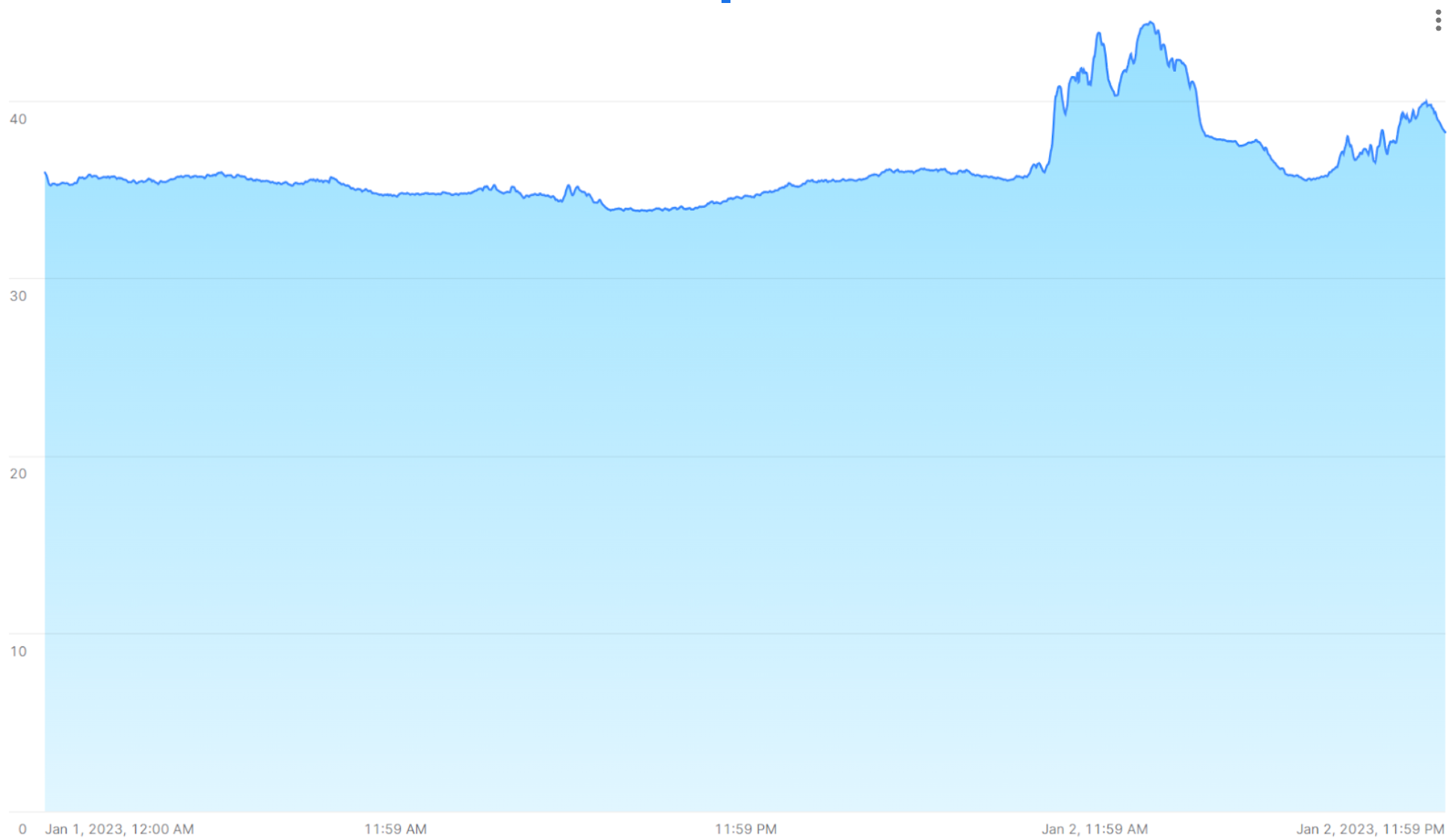
A time series might reveal spikes when readings change dramatically for some reason. For example, the following image shows a sequence of temperature readings taken at 15-second intervals, with values peaking over 40°C after being steadily in the 35°C range for the previous day.
The following sections show how to analyze and visualize large volumes of this kind of data with SQL functions and joins that provide fast, accurate results.
How to store time-series data
The following datetime data types are supported:
- DATE
- TIME
- TIMESTAMP (and variations, including TIMESTAMP_TZ)
For information about loading, managing, and querying data that uses these data types, see Working with date and time values.
A number of commonly used SQL functions are available to help with both storing and querying time-series data. For example, you can use CONVERT_TIMEZONE to convert timestamps from one time zone to another, and you can use functions such as EXTRACT and TIMEADD to manipulate time-based data as needed.
Note
For TIMESTAMP_TZ data, Snowflake stores the offset of a given time zone, not the actual time zone, at the moment of creation for a given value.
To optimize query performance, tables used for time-series analytics are often clustered by time (and sometimes also by sensor ID or a similar dimension). See Clustering Keys & Clustered Tables.
Aggregating time-series data
Management of time-series data might require the aggregation of large volumes of fine-grained records into a more summarized form (a process sometimes referred to as “downsampling”). Given a large set of records with a specific time-based granularity (milliseconds, seconds, minutes, etc.), you can roll up these records to a coarser granularity, effectively producing a smaller sample.
Downsampling is valuable because it decreases the size of a data set and its storage requirements. A coarser level of granularity also reduces compute resource requirements during query execution. Another key reason for downsampling is that a large number of records in a time series might be redundant from an analyst’s point of view. For example, if a sensor emits a new value once every second, but this measurement rarely changes within each 60-second interval, the data can be rolled up to the minute level for analysis.
Another case for downsampling occurs when two different data sets need to be analyzed as one, but they have different time granularities. For example, Sensor A in a factory collects data every 15 seconds, but Sensor B collects related data every 30 seconds. In this case, aggregating the records into 1-minute buckets might be a good solution. IDs and dimensions in each data set are retained as they are, but numeric measurements are summed or averaged by a common time interval.
Downsampling examples
You can downsample a data set that is stored in a table by using the TIME_SLICE function. This function calculates the start and end times of fixed-width “buckets” so that individual records can be grouped and summarized, using standard aggregate functions, such as SUM and AVG.
Similarly, the DATE_TRUNC function truncates part of a series of date or timestamp values, reducing their granularity. The following sections show examples of each function.
Downsampling with TIME_
The following example downsamples a table named sensor_data_ts, which contains readings
from two factory sensors and contains 5.3 million rows. These readings were ingested per second, so 5.3 million rows
represents only one month of data, with just over 2.5 million rows per sensor. You can use the TIME_SLICE function to
aggregate up to a single row per minute, per hour, or per day, for example.
To run this example, first create and load the sensor_data_ts table; see Creating the sensor_data_ts table.
Here is a small sample of the data in the table:
The table contains 60 readings like these per minute for each device, as shown by this query:
In this downsampling query, the TIME_SLICE function defines one-minute buckets and returns the start time of each bucket. The AVG function calculates the average temperature for each bucket per device. The COUNT(*) function is included for reference, just to show how many rows land in each time bucket.
The vibration and motor_rpm columns are not included, but they could be aggregated in the same way
as the temperature column or by using different aggregate functions.
Important
If you run this example yourself, your output will not match exactly because the sensor_data_ts table is loaded
with randomly generated values.
By using the TIME_SLICE function, you can create smaller, aggregated tables for analysis purposes, and you can apply the downsampling process at different levels (hour, day, week, and so on).
Downsampling with DATE_
The following example selects data from a table named order_header in the raw.pos
schema of the
Tasty Bytes sample database.
This table contains 248M rows.
The order_header table has a TIMESTAMP column named order_ts. The query creates an aggregated time series by
using this column as the second argument to the DATE_TRUNC function. The first argument specifies a day interval.
This means that the individual records, which have an hours/minutes/seconds granularity, are rolled up by day.
The query groups the records by two dimensions: truck_id and
location_id. The avg_amount column returns the average price per order, per food truck, per
location for each business day on record.
The query shown here limits the results to the first 25 rows for January 1, 2022. If you remove this date filter and the LIMIT clause, the query downsamples the original 248M rows to about 500,000 rows.
Using windowed aggregations for rolling calculations
By using windowed aggregate functions to observe how a metric changes over time, you can analyze a time series for trends. Windowed aggregations are useful for analyzing data within defined subsets (“windows”) of a larger data set. You can compute rolling calculations (such as moving averages and sums) for each row in a data set, taking into account a group of rows before, after, or surrounding the current row. This kind of analysis contrasts with regular aggregations, which summarize the entire data set.
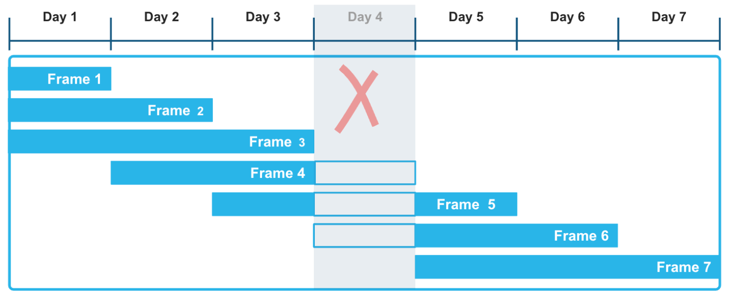
By using range-based window frames with explicit offsets, you can apply a very flexible approach to computing
these rolling aggregations. The RANGE BETWEEN window frame, ordered by either timestamps or numbers, is not disrupted
by gaps that may occur in time-series data. For instance, in the following illustration, the fact that Day 4
data is missing in the series of records does not affect the computation of aggregate functions over a three-day moving
window. In particular, frames 3, 4, and 5 are computed correctly, taking into account that Day 4 data is unknown.
The following example calculates a moving sum over weather data that records hourly precipitation readings in different cities and counties. You can run this kind of query to evaluate trends in various time-series data sets, such as sensors and other IoT devices, especially when those data sets are known or expected to have gaps.
The window function includes in its frame the current precipitation reading and all the readings that fall within the
specified time interval before the current reading. The rolling calculation is based on this flexible and
logical range of rows rather than an exact number of rows. The first row for each city has matching precip and
moving_sum_precip values. After that, the sum is recalculated for each subsequent row in the frame. The raw values
fluctuate significantly, but the moving sums have a strong smoothing effect.
To run this example, follow these instructions first: Create and load the heavy_weather table.
This very small table contains sporadic hourly weather observations, with lots of gaps, including a missing day. The query
returns the moving sum of precipitation values ordered by the start_time column. The window frame defines a
range between 12 hours before the current row and the current row. Therefore, the frame consists of the current row plus only those
rows that have timestamps up to 12 hours earlier than the ORDER BY timestamp for the current row.
The three moving_sum_precip values for Big Bear City are calculated as follows:
- 0.42 = 0.42 (no preceding rows)
- 0.42 + 0.09 = 0.51 (the first two rows are within the 12-hour window)
- 0.07 = 0.07 (no preceding rows are within the 12-hour window)
The South Lake Tahoe rows include these calculations, for example:
- 0.56 + 0.38 + 0.28 + 0.80 = 2.02 (all four rows for 2024-12-23 are within 12 hours of each other)
- 0.80 + 0.17 = 0.97 (one preceding row is within the 12-hour window)
Other window functions, such as the LEAD and LAG ranking functions, are also commonly used in time-series analysis. Use the LEAD window function to find the next data point in the time series, relative to the current data point, and the LAG function to find the previous data point.
Visualizing query results in Snowsight
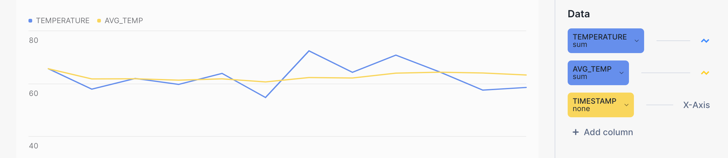
You can use Snowsight to visualize the results of aggregation queries, and get a better sense of the smoothing effect of calculations with sliding window frames. In the query worksheet, click the Chart button next to Results.
For example, the yellow line in the following bar chart shows a much smoother trend for average temperature versus the blue line for the raw temperature. The query itself looks like this:
Using the MIN_
The ability to select one column based on the minimum or maximum value of another column in the same row is a common requirement for SQL developers who are working with time-series data. MIN_BY and MAX_BY are convenience functions that return the starting and ending (or highest and lowest, or first and last) values in a table when the data is sorted by some other column, such as a timestamp.
The first example simply finds the last (most recent) precip value in the whole table. The MAX_BY function sorts all the rows
by their start_time value, then returns the precip value for the “max” start time.
To create and load the table used in the following examples, see Creating the heavy_weather table.
You can verify this result (and get more information about it) by running this query:
You can add a GROUP BY clause to ask more interesting questions about this data. For example, the following query
finds the last precipitation value that was observed for each city in California, ordered by precip values
(high to low). The results are grouped by city to return the last precip value for each different city.
The last time an observation was taken for the city of Alta, the precip value was 0.89,
and the last time an observation was taken for the cities of South Lake Tahoe, Big Bear City, Montague, and Lebec, the precip
value was 0.07 for all four locations. (Note that the query does not tell you when those observations were taken.)
You can return the “opposite” result set (oldest precip record versus most recent) by using the MIN_BY function.
Joining time-series data
You can use the ASOF JOIN construct to join tables that contain time-series data. Although ASOF JOIN queries can be emulated through the use of complex SQL, other types of joins, and window functions, these queries are easier to write (and are optimized) if you use the ASOF JOIN syntax.
A common use for ASOF joins is the analysis of financial trading data. Transaction-cost analysis, for example, requires “slippage” calculations, which measure the difference between the price quoted at the time of a decision to buy stocks and the price actually paid when the trade was executed and recorded. The ASOF JOIN can expedite this type of analysis. Given that the key capability of this join method is the analysis of one time series with respect to another, ASOF JOIN can be useful for analyzing any data set that is historical in nature. In many of these use cases, ASOF JOIN can be used to associate data when readings from different devices have timestamps that are not exactly the same.
The assumption is that the time-series data you need to analyze exists in two tables, and there is a timestamp for each row in each table. This timestamp represents the precise “as of” date and time for a recorded event. For each row in the first (or left) table, the join uses a “match condition” with a comparison operator that you specify to find a single row in the second (or right) table where the timestamp value is one of the following:
- Less than or equal to the timestamp value in the left table.
- Greater than or equal to the timestamp value in the left table.
- Less than the timestamp value in the left table.
- Greater than the timestamp value in the left table.
The qualifying row on the right side is the closest match, which could be equal in time, earlier in time, or later in time, depending on the specified comparison operator.
The cardinality of the result of the ASOF JOIN is always equal to the cardinality of the left table. If the left table contains 40 million rows, the ASOF JOIN returns 40 million rows. Therefore, the left table can be thought of as the “preserving” table, and the right table as the “referenced” table.
Joining two tables on the closest match (alignment)
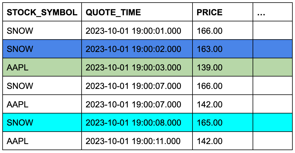
For example, in a financial application, you might have a table named quotes and a table named trades.
One table records the history of bids to buy stock, and the other records the history of actual trades.
A bid to buy stocks happens before the trade (or possibly at the “same” time, depending on the granularity of
the recorded time). Both tables have timestamps, and both have other columns of interest that you might want to
compare. A simple ASOF JOIN query will return the closest quote (in time) before each trade. In other words,
the query asks: What was the price of a given stock at the time I made a trade?
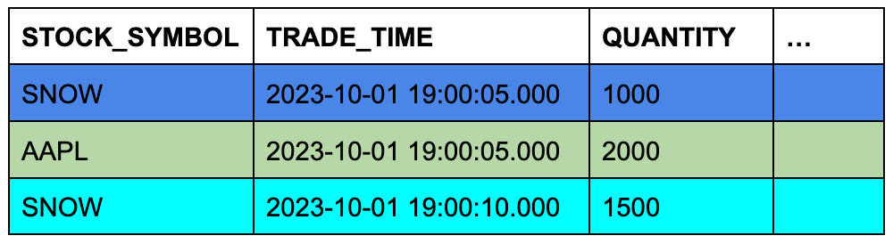
Assume that the trades table contains three rows, and the quotes table contains seven rows.
The background color of the cells shows which three rows from quotes will qualify for the ASOF JOIN when the
rows are joined on matching stock symbols and their timestamp columns are compared.
TRADES Table (Left or “Preserving” Table)
QUOTES Table (Right or “Referenced” Table)
This conceptual example is easy to turn into a specific ASOF JOIN query:
The ON condition groups the matched rows by their stock symbols.
To run this example, create and load the tables as follows:
For more examples of ASOF JOIN queries, see Examples.
Filling gaps in time-series data
Time-series analysis often requires data to have a consistent granularity with records for every interval, yet real-world data often arrives at irregular intervals or contains gaps. For instance, you might have a predominantly hourly data set but need to generate half-hour entries to align with downstream analytics, or you might already have a consistent resolution but discover gaps in the series. Snowflake gap-filling functionality provides efficient ways to apply a uniform interval to time-series data and fill any gaps.
For example, consider the following eight records, which capture weather observations for two cities in California on March 15, 2025.
Although these records have a somewhat consistent level of granularity (day, hour, minute), the intervals between the rows are inconsistent, varying between 1 and 15 minutes. If the goal is to collect data at five-minute intervals, several rows are missing.
Using the RESAMPLE clause
You can modify the granularity and improve the consistency of a set of rows by “upsampling” them to a specific time interval. To make this kind of change, use the RESAMPLE clause, which you define within the FROM clause of a SELECT statement. The result of a resampled data set is a larger data set that preserves all of the existing input rows and generates some number of new rows with values that fill gaps in the time series. (Note that you can also use the RESAMPLE clause to “downsample” rows into a smaller, more coarse-grained result set.)
By definition, a time series always has a column that contains a sequence of dates, timestamps, or numeric values that represent dates or times.
Resampling operates on such a column in the source table, and the required granularity must be specified with an INTERVAL value, such as
5 minutes, 30 minutes, or 1 hour.
Typically, you also define partitions that create time-series rows over certain dimensions, rather than just generating one new timestamp per interval.
The structure of a RESAMPLE query looks like this:
Columns in the rows that are generated are set to NULL, except for the columns specified in the USING and PARTITION BY clauses. The specified date, time, or numeric column and the partitioning columns have meaningful generated values.
Note
If you plan to filter your resampled data by specific values (for example, a specific device ID or location), include those columns in the PARTITION BY clause. This ensures that generated rows have real values for those columns rather than NULL values. If you filter with a WHERE clause on columns that are not in the PARTITION BY clause, the WHERE clause filters out all generated rows for those columns because they contain NULL values.
To run a simple example that uses the eight records shown earlier, start by creating and loading the following table:
Now select upsampled rows from that table, using an interval of 5 minutes:
This query preserves the original eight rows and generates three new rows, filling gaps for three time intervals, at 09:45, 10:00, and 10:05.
NULL values are inserted into the temperature, city, and county columns.
The starting point for the time series is 2025-03-15 09:45:00.000 because it is within 5 minutes of the earliest timestamp in the input data set
(2025-03-15 09:49:00.000).
If you want to remove rows that don’t occur at uniform intervals (09:49 and 10:18 in this case), see RESAMPLE example that uses BUCKET_START() to filter out non-uniform rows.
Now add a PARTITION BY clause to the query:
The partitioned results are different in two ways:
- Seven rows are generated, for a total of 15 rows. A row now exists for every 5-minute interval for every partition.
- The partitioning columns have correctly generated
cityandcountyvalues. The only column that has NULL values in the generated rows istemperature.
You can also specify the METADATA_COLUMNS parameter in the RESAMPLE syntax to add the following columns to the result:
- The
is_generatedmetadata column identifies the rows that were generated by the RESAMPLE operation and the rows that were already present. - The
bucket_startmetadata column returns the value that marks the beginning of the current bucket or interval that the RESAMPLE operation produces. You can use this column to identify which interval a particular row belongs to after resampling, and you can use it to run aggregate queries on resampled data. See RESAMPLE example that uses BUCKET_START() to aggregate resampled rows.
For the complete RESAMPLE syntax, see RESAMPLE.
To store the results of a RESAMPLE query, use a CTAS statement that selects and inserts the data into a new table:
Interpolating or “gap-filling” values into a time series
Although you can use the RESAMPLE syntax and interpolation functions independently, they are most commonly used together to gap-fill time-series data in the scope of a single query. Having resampled your data set, you can call an interpolation function to update the other columns of interest in the newly generated rows. The interpolation process updates columns that were previously NULL, such as numeric measurements, giving them meaningful values based on values found in the preceding or following rows.
You can interpolate values by calling the INTERPOLATE_FFILL, INTERPOLATE_BFILL, and INTERPOLATE_LINEAR window functions. For example, the INTERPOLATE_FFILL function finds the previous (last) value in the time series for the column in question:
The first row returns NULL for the ffill_temp column because there is no previous row for the INTERPOLATE_FFILL function to use.
For more information about these window functions, see INTERPOLATE_BFILL, INTERPOLATE_FFILL, INTERPOLATE_LINEAR.
Upsampling, gap-filling, and storing the results in one operation
To simplify the whole process of gap-filling a data set, you can upsample data and interpolate values within a single query, and save the results by using a CTAS operation. For example, the following CTAS statement creates a new table that interpolates measurements into a an upsampled data set:
Note
When you use INTERPOLATE functions with resampling, the columns you specify in the OVER (PARTITION BY) clause for window functions typically match
the columns in the RESAMPLE (PARTITION BY) clause. This approach ensures that interpolation happens within the same logical partitions that were created
during resampling. In the previous example, resampling is partitioned by city and county, while the INTERPOLATE functions partition by city only.
This example works because the interpolation is happening at a coarser granularity, but you should always make sure that the partitioning strategy aligns with your data requirements.
Gap-filling with ASOF JOIN
Note
To use the recommended approach for gap-filling and interpolation, see Filling gaps in time-series data. The RESAMPLE construct and INTERPOLATE functions are preview features, and the following ASOF JOIN approach to gap-filling is included only as a potential workaround.
In addition to aligning the data in two tables by finding non-exact matches on time-based columns, ASOF JOIN is useful for filling gaps in a time series when your raw data table is missing rows for particular dates or timestamps. For example, when rows are missing because faulty equipment, or a power failure, results in skipped sensor readings, you can use ASOF JOIN to interpolate values from a generated time series into the table. The missing rows are filled in with the last known value for the readings that are missing. This value is also known as the “last observation carried forward” (LOCF). The ASOF JOIN query returns a complete set of rows that are in chronological order and contiguous.
To use ASOF JOIN for interpolation, follow these steps:
-
Identify the gaps in your table by running a simple query.
-
Generate a complete time series, with the appropriate grain, for the period of time that you need to cover. For example, your time series might be a simple sequence of dates for a particular year, or a much more granular sequence of timestamps per second for some number of days. You can use SQL or a spreadsheet application to generate the list of values.
The time series will also need a meaningful ID or dimension for each row that you will specify later in the ASOF JOIN ON condition.
-
Write an ASOF JOIN query that interpolates values into the missing rows. The generated time series will be the preserving table and the raw data table will be the referenced table.
The following example requires the sensor_data_ts table. If you haven’t already created and loaded it, see
Creating the sensor_data_ts table. To simulate the need for a gap-filling operation, delete some rows from the table as follows:
The result is a table that is missing five rows for DEVICE2 on March 7th (1:16 through 1:20).
Now follow these steps to complete the gap-filling exercise.
Note
If you run this example yourself, your output will not match exactly because the sensor_data_ts table is loaded
with randomly generated values.
Step 1: Verify that the table has gaps
Run the following query to identify the gaps:
This query returns two rows for DEVICE2: the last row before the gap and the first row
after the gap.
Step 2: Generate a complete time series to cover the known gaps
To generate a time series with a fine grain (one row per second) for the gap in the sensor_data_ts
table, create the following table, which contains generated timestamps:
In this SQL statement, 5 is the number of seconds that you need to cover the gap. Note that the device ID value
(DEVICE2) is included in the generated rows.
The following query returns the five generated rows.
Step 3: Interpolate values by using ASOF JOIN
Now you can run an ASOF JOIN query that joins continuous_timestamps to sensor_data_ts and
interpolates values for missing rows for DEVICE2. The match condition finds the closest
row in time for each missing row, and the ON condition guarantees that interpolation occurs
on matching device IDs.
The closest row for the missing rows is the row with the 2024-03-07 00:01:16.000 timestamp,
assuming that >= is specified in the match condition, as shown in this example.
This INSERT statement selects five rows from the ASOF JOIN operation and inserts them into the
sensor_data_ts table.
To check the results of the interpolation, select those five rows, and the two rows that directly precede and
follow them, from the sensor_data_ts table. Note that the five interpolated rows have picked up the same values
for the temperature, vibration, and motor_rpm columns that were recorded in the 2024-03-07 00:01:15.000
row. The interpolation was successful.
Applying ML-based functions to time-series data
You can train a model with ML Functions to do predictive analysis on time-series data:
Forecasting uses historical time-series data to make predictions about future data. Given a recorded time series with actual observed values for dates and times in the past, the ML model forecasts what the observed values might be for dates and times in the future.
Anomaly detection identifies outliers, which are data points that deviate from an expected range. In the context of a time series, an outlier is a measurement that is much larger or smaller than other measurements in a similar time interval. To find outliers, the ML function produces a forecast for the same time period that is being checked for anomalies, then compares the forecast results to the actual data.
Top Insights finds the most important dimensions in a data set, builds segments from those dimensions, and detects which of those segments influenced a metric.
Note
For machine-learning purposes, the timestamps in your time series must represent fixed time intervals. If necessary, you can use the DATE_TRUNC or TIME_SLICE function on TIMESTAMP columns to remove irregularities when training the forecast model.
An example of anomaly detection in a time series
The following example uses a view with only 30 rows to train an anomaly detection model. Start by generating data into a table, then create a view on the table. The view is not required (you can use a table to train a model), but the view option gives you some flexibility to train models iteratively, with different row counts, without updating the source data.
Note
If you run this example yourself, your output will not match exactly because the sensor_data_30_rows table is loaded
with randomly generated values.
Now create the model:
When the model has built successfully, call the <model_name>!DETECT_ANOMALIES method to detect outliers in the specified test data set. The timestamps in the test data must chronologically follow the timestamps in the training data, but there must not be too great a gap in time between the training data and the test data. For example, if you have timestamps for every second, do not use test data that is millions of seconds ahead of the training data.
This example uses another table as the test data, with only three rows. These rows have timestamps that closely follow those in the training data.
When the anomaly detection call finishes, it returns output similar to the following:
The TS and Y columns return the timestamps and temperature values from the test data. In this very small test case,
the function found an anomaly (IS_ANOMALY=True). For more information about the output columns, see the “Returns” section in the
function description.
Creating the sensor_
If you want to test the examples in this section that query the sensor_data_ts table, you can create and load
a copy of this table by running the following SQL script. The script generates one month of synthetic data for sensor
readings by calling the UNIFORM, RANDOM, and GENERATOR functions; therefore, your copy of the table will not return identical
results. The readings will be in the same range but they will not be the same.
Creating the heavy_
The following script creates and loads the heavy_weather table, which is used in the examples
for the MAX_BY functions. The table contains 55 rows of snowfall precipitation records for
California cities during the last week of 2021.