Micro-partitions & Data Clustering
Traditional data warehouses rely on static partitioning of large tables to achieve acceptable performance and enable better scaling. In these systems, a partition is a unit of management that is manipulated independently using specialized DDL and syntax; however, static partitioning has a number of well-known limitations, such as maintenance overhead and data skew, which can result in disproportionately-sized partitions.
In contrast to a data warehouse, the Snowflake Data Platform implements a powerful and unique form of partitioning, called micro-partitioning, that delivers all the advantages of static partitioning without the known limitations, as well as providing additional significant benefits.
Attention
Hybrid tables are based on an architecture that does not support some of the features that are available in standard Snowflake tables, such as clustering keys.
What are Micro-partitions?
All data in Snowflake tables is automatically divided into micro-partitions, which are contiguous units of storage. Each micro-partition contains between 50 MB and 500 MB of uncompressed data (note that the actual size in Snowflake is smaller because data is always stored compressed). Groups of rows in tables are mapped into individual micro-partitions, organized in a columnar fashion. This size and structure allows for extremely granular pruning of very large tables, which can be comprised of millions, or even hundreds of millions, of micro-partitions.
Snowflake stores metadata about all rows stored in a micro-partition, including:
- The range of values for each of the columns in the micro-partition.
- The number of distinct values.
- Additional properties used for both optimization and efficient query processing.
Note
Micro-partitioning is automatically performed on all Snowflake tables. Tables are transparently partitioned using the ordering of the data as it is inserted/loaded.
Benefits of Micro-partitioning
The benefits of Snowflake’s approach to partitioning table data include:
- In contrast to traditional static partitioning, Snowflake micro-partitions are derived automatically; they don’t need to be explicitly defined up-front or maintained by users.
- As the name suggests, micro-partitions are small in size (50 to 500 MB, before compression), which enables extremely efficient DML and fine-grained pruning for faster queries.
- Micro-partitions can overlap in their range of values, which, combined with their uniformly small size, helps prevent skew.
- Columns are stored independently within micro-partitions, often referred to as columnar storage. This enables efficient scanning of individual columns; only the columns referenced by a query are scanned.
- Columns are also compressed individually within micro-partitions. Snowflake automatically determines the most efficient compression algorithm for the columns in each micro-partition.
You can enable clustering on specific tables by specifying a clustering key for each of those tables. For information about specifying a clustering key, see:
For additional information about clustering, including strategies for choosing which tables to cluster, see:
Impact of Micro-partitions
DML
All DML operations (e.g. DELETE, UPDATE, MERGE) take advantage of the underlying micro-partition metadata to facilitate and simplify table maintenance. For example, some operations, such as deleting all rows from a table, are metadata-only operations.
Dropping a Column in a Table
When a column in a table is dropped, the micro-partitions that contain the data for the dropped column are not re-written when the drop statement is executed. The data in the dropped column remains in storage. For more information, see the usage notes for ALTER TABLE.
Query Pruning
The micro-partition metadata maintained by Snowflake enables precise pruning of columns in micro-partitions at query run-time, including columns containing semi-structured data. In other words, a query that specifies a filter predicate on a range of values that accesses 10% of the values in the range should ideally only scan 10% of the micro-partitions.
For example, assume a large table contains one year of historical data with date and hour columns. Assuming uniform distribution of the data, a query targeting a particular hour would ideally scan 1/8760th of the micro-partitions in the table and then only scan the portion of the micro-partitions that contain the data for the hour column; Snowflake uses columnar scanning of partitions so that an entire partition is not scanned if a query only filters by one column.
In other words, the closer the ratio of scanned micro-partitions and columnar data is to the ratio of actual data selected, the more efficient is the pruning performed on the table.
For time-series data, this level of pruning enables potentially sub-second response times for queries within ranges (i.e. “slices”) as fine-grained as one hour or even less.
Not all predicate expressions can be used to prune. For example, Snowflake does not prune micro-partitions based on a predicate with a subquery, even if the subquery results in a constant.
What is Data Clustering?
Typically, data stored in tables is sorted/ordered along natural dimensions (e.g. date and/or geographic regions). This “clustering” is a key factor in queries because table data that is not sorted or is only partially sorted may impact query performance, particularly on very large tables.
In Snowflake, as data is inserted/loaded into a table, clustering metadata is collected and recorded for each micro-partition created during the process. Snowflake then leverages this clustering information to avoid unnecessary scanning of micro-partitions during querying, significantly accelerating the performance of queries that reference these columns.
The following diagram illustrates a Snowflake table, t1, with four columns sorted by date:
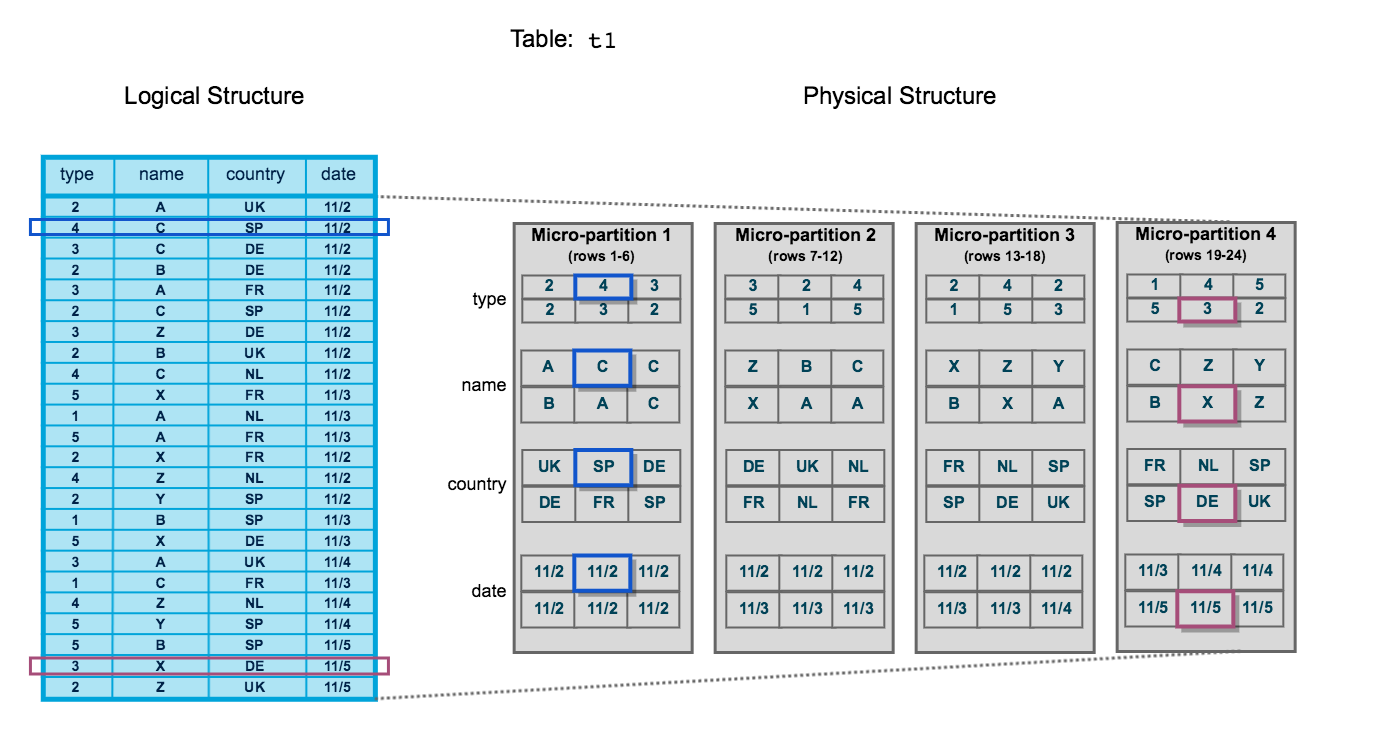
The table consists of 24 rows stored across 4 micro-partitions, with the rows divided equally between each micro-partition. Within each micro-partition, the data is sorted and stored by column, which enables Snowflake to perform the following actions for queries on the table:
- First, prune micro-partitions that are not needed for the query.
- Then, prune by column within the remaining micro-partitions.
Note that this diagram is intended only as a small-scale conceptual representation of the data clustering that Snowflake utilizes in micro-partitions. A typical Snowflake table may consist of thousands, even millions, of micro-partitions.
Clustering Information Maintained for Micro-partitions
Snowflake maintains clustering metadata for the micro-partitions in a table, including:
- The total number of micro-partitions that comprise the table.
- The number of micro-partitions containing values that overlap with each other (in a specified subset of table columns).
- The depth of the overlapping micro-partitions.
Clustering Depth
The clustering depth for a populated table measures the average depth (1 or greater) of the overlapping micro-partitions for specified columns in a table. The smaller the average depth, the better
clustered the table is with regards to the specified columns.
Clustering depth can be used for a variety of purposes, including:
- Monitoring the clustering “health” of a large table, particularly over time as DML is performed on the table.
- Determining whether a large table would benefit from explicitly defining a clustering key.
A table with no micro-partitions (i.e. an unpopulated/empty table) has a clustering depth of 0.
Note
The clustering depth for a table is not an absolute or precise measure of whether the table is well-clustered. Ultimately, query performance is the best indicator of how well-clustered a table is:
- If queries on a table are performing as needed or expected, the table is likely well-clustered.
- If query performance degrades over time, the table is likely no longer well-clustered and may benefit from clustering.
Clustering Depth Illustrated
The following diagram provides a conceptual example of a table consisting of five micro-partitions with values ranging from A to Z, and illustrates how overlap affects clustering depth:
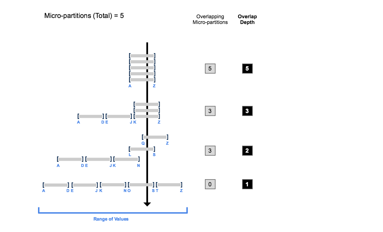
As this diagram illustrates:
- At the beginning, the range of values in all the micro-partitions overlap.
- As the number of overlapping micro-partitions decreases, the overlap depth decreases.
- When there is no overlap in the range of values across all micro-partitions, the micro-partitions are considered to be in a constant state (i.e. they cannot be improved by clustering).
The diagram is not intended to represent an actual table. In an actual table, with data contained in a large numbers of micro-partitions, reaching a constant state across all micro-partitions is neither likely nor required to improve query performance.
Monitoring Clustering Information for Tables
To view/monitor the clustering metadata for a table, Snowflake provides the following system functions:
- SYSTEM$CLUSTERING_DEPTH
- SYSTEM$CLUSTERING_INFORMATION (including clustering depth)
For more details about how these functions use clustering metadata, see Clustering Depth Illustrated (in this topic).